General Tutorial
Overview
This tutorial explains how to complete a series of typical tasks for data entry, reporting and analysis. When you have completed this tutorial, you will have gained enough skills to begin entering and importing data from a range of sources, and generating reports.
gINT Program Overview
- Overview of gINT Features and Capabilities
- Database manager for subsurface exploration
- Storing, validating, manipulating and reporting data
- Graphic Tools available in gINT
- gIDraw
- Symbols
- Grid Input and Graphical Data Input
- How gINT communicates with other programs
- Data import and export
- Graphical import and export
- gINT's Application Groups and layout of program:
- Input
- Output
- Data Design
- Report Design
- Symbol Design
- Drawings
- Utilities
- gINT Products
- Logs
- Professional
- Professional Plus
- gINT Civil Tools
- Bentley SES license system
- Help menu
Preliminary settings
- Install and license gINT and the DGDT DLL program.
- For the tutorial copy the dgdt user gINT files (*.gpj, *.gdt, *.glb, *.gcx, *.gci, *.gas) to a folder titled c:\Datgel Training\.
- Open gINT.
- Open the dgdt-p lib #.##.#.glb library using the command File > Change Library. If you are running an evaluation or trial version, the library is read-only and the design applications are hidden.
- Launch File > System Properties, and configure the following on the first tab.
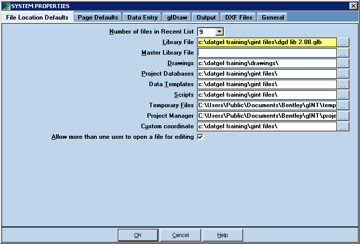
- Refer to section Configure Optimal System Properties for further instruction.
Data entry of a borehole
Make a new project by cloning data template
To make a new Access Project File:
- Select INPUT | File > New Project or the (new) icon > Clone Data Template…
- Browse to the data template dgdt-p #.##.#.gdt, and click Open.
- Name the new project file Tutorial.gpj, and click Save.
General
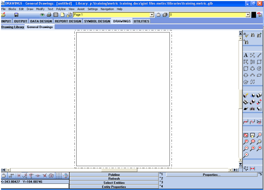
Progress through the INPUT application entering data displayed in the screen shots.
You can change tables or tabs by clicking on the tabs at the top of the screen or using the tree navigation on the left. To enable and disable the tree navigation click on the button: ![]() .
.
Data is saved when you initiate the save by clicking on the save icon, pressing Ctrl+S, or automatically when you change tabs, or change the object selector item (yellow drop down list), or before some commands run. It is recommended that you save data after entering a few lines.
There is not a multi step undo like in Word. The closest option is Cancel changes since last save, which is the save like icon with the red arrow in the top right of the screen.
Project
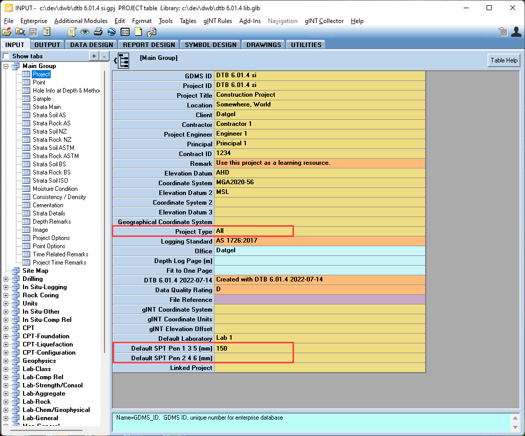
Set the Project Type and SPT Pen Values to match you standard. If you are using BS, then both SPT Pen fields should be 75, other standards should have 150 and empty cell.
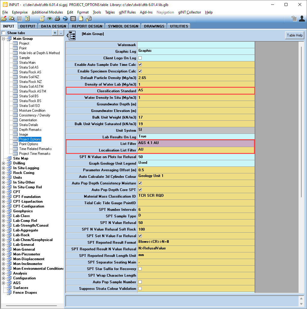
Project Options
- The settings on this table generally depend upon the logging standards in use, and it is critical the relevant values are set for Classification_Standard, List_Filter and Localisation_List_Filter.
- Enable Specimen Description Calc – check
- Note the Graphic Log option controls the log report column, set it to Graphic.
Point
- Use Tab or right arrow to move to the next cell.
- Press F2 to make a cell editable.
- Press Ctrl+Enter to move to next line.
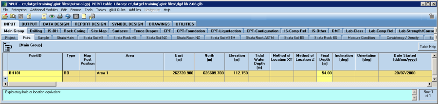
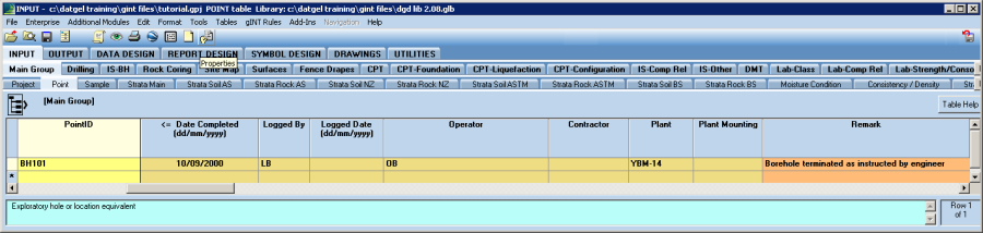
- To rename a PointID, change the name in the POINT table PointID field.
- Set Depth Borehole / Corehole Break, to define the depth that the non cored log ends and cored log starts
Strata Main
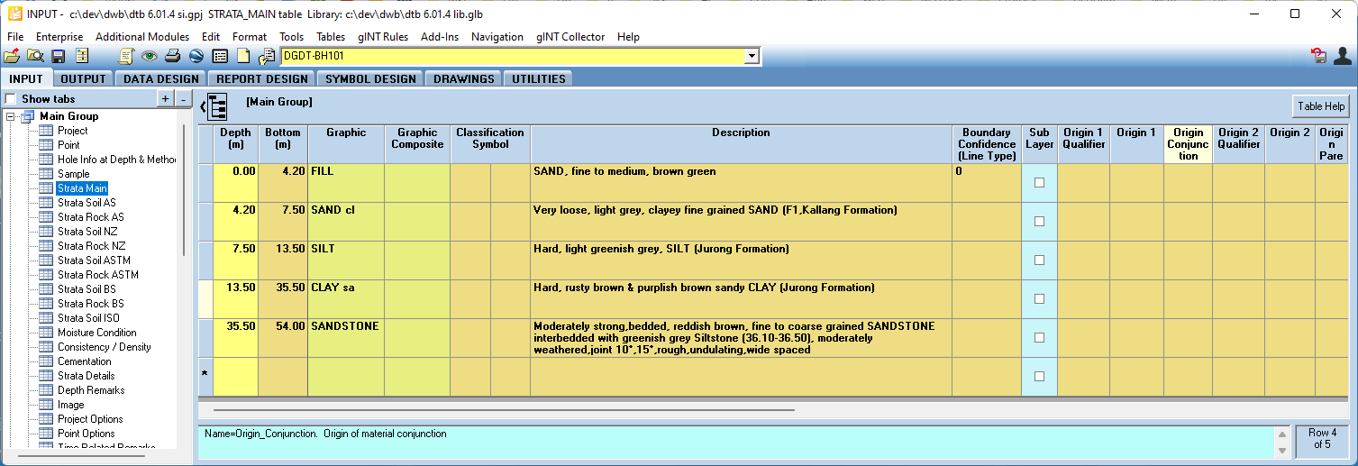
Speed up selection by using lookup lists. F2 makes the list expand. If you type into fields, matching items are selected automatically.
If you follow Australian or New Zealand practice, at this point you'd enter data into tables:
- Main Group | Moisture Condition
- Main Group | Consistence/Density
- Rock Coring | Rock Strength
- Rock Coring | Weathering
- Rock Coring | Defects
- Rock Coring | Fractures
Component Description tables
The DGDT incorporates component description tables for AS, NZGS, BS and ASTM. Data in the component description tables will be displayed in priority over data in Stata Main.
Enter one description in the component description tables for soil and rock that best matches the standard you log to.
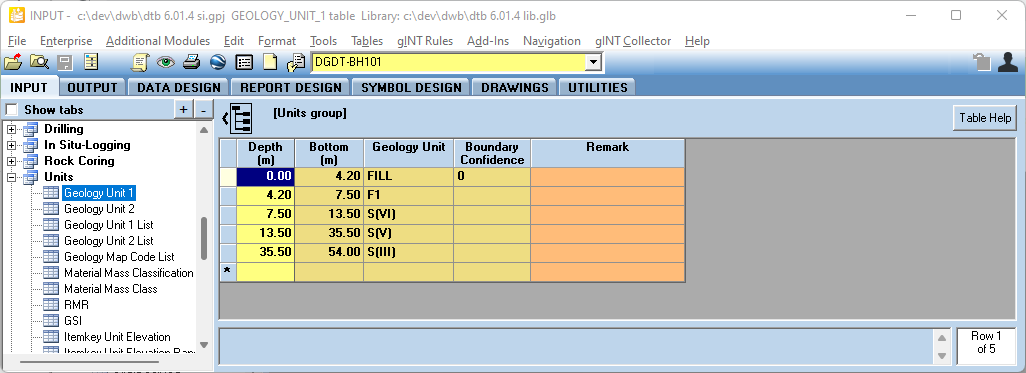
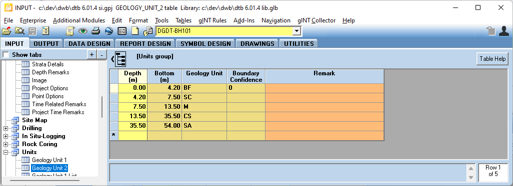
Geology Unit
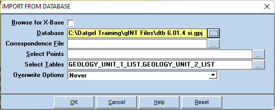
You will find the Geology Unit 1 and 2 lookup lists empty. In this example a standard list of units from Singapore is applicable, and these can be imported from the example project dgdt-p #.##.#.gpj. Select File > Import/Export > Import from Database…, and configure the options as in the following screen shot, then click OK.
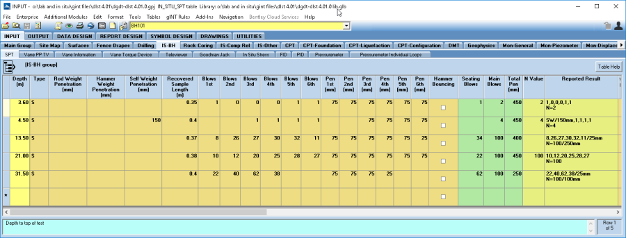
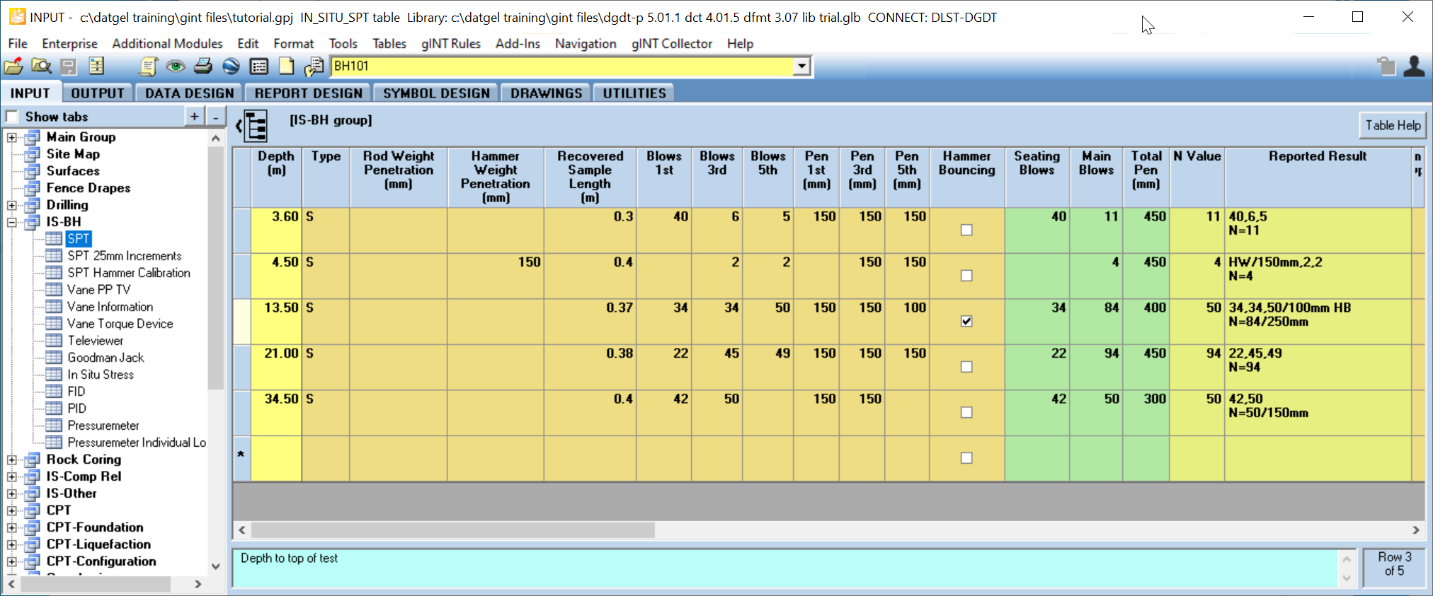
SPT
- Do not enter data in the green fields, these will calculate when the grid saves.
- If your logging standard uses 3 intervals, then enter data in columns 1, 3, and 5.
- If you enter a Recovered_Sample_Length, then a corresponding record will be created on the Sample table.
BS
AS / NZGS / ASTM
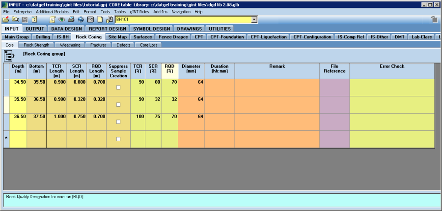
Core
- Enter data in the Length fields, and the result fields will be calculated.
- Unless you check the box, corresponding same records will be made.
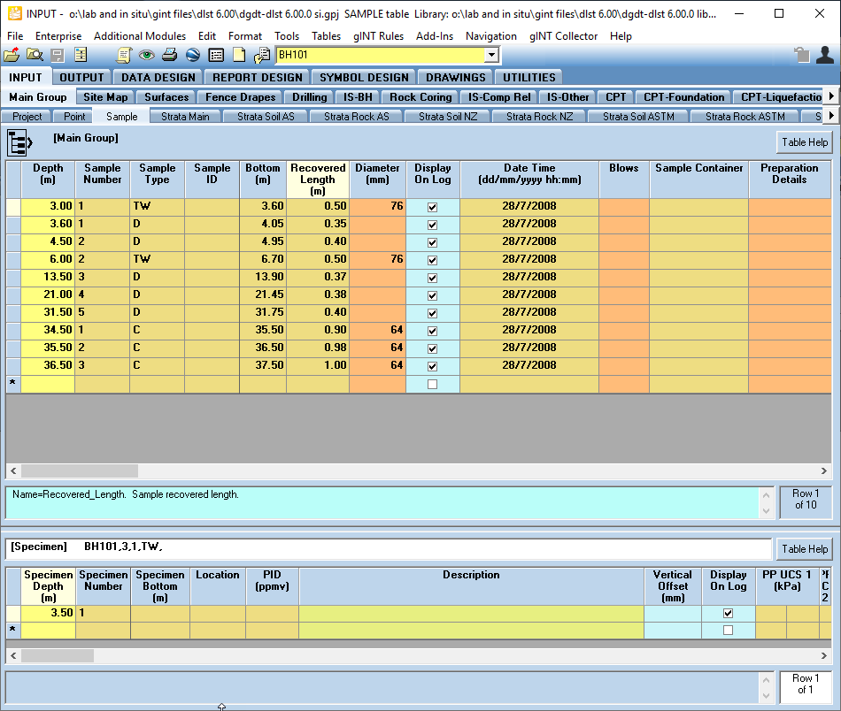
Sample
Other than the TW type records, the data was automatically created by the DGDT program. You can edit the data without it being overwritten, since the same function only runs when new records are created on the SPT and Core tables.
Other common logging tables
At this point you may like to enter data for these tables
- Method, Shoring, Hole Info at Depth
- Water Strike/Inflow
- Progress & Drilling Fluid Levels
- Rotary Flush
- Point Load Strength, which is under Lab-Rock. See Lab data entry section below.
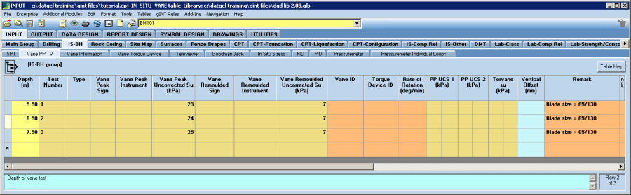
Shear Vane
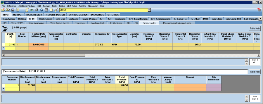
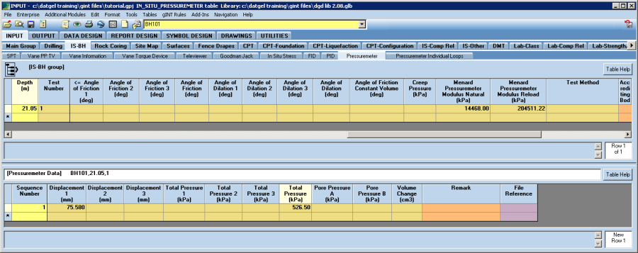
Pressuremeter
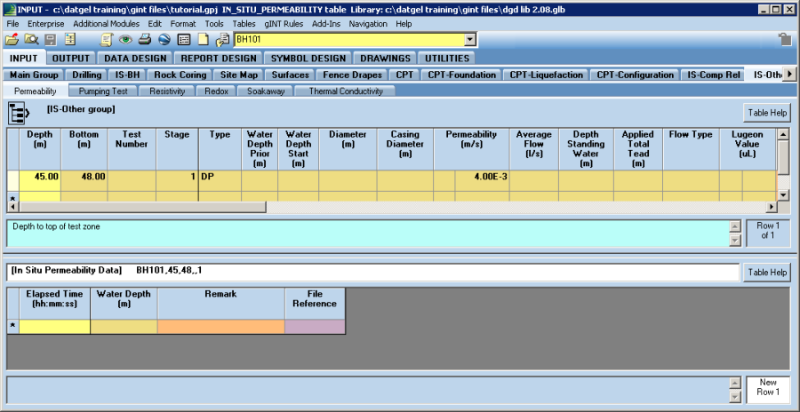
In Situ Permeability
Piezometer data entry
The DGD Tool allows the storage of piezometer data and includes log reports that display piezometer installation.
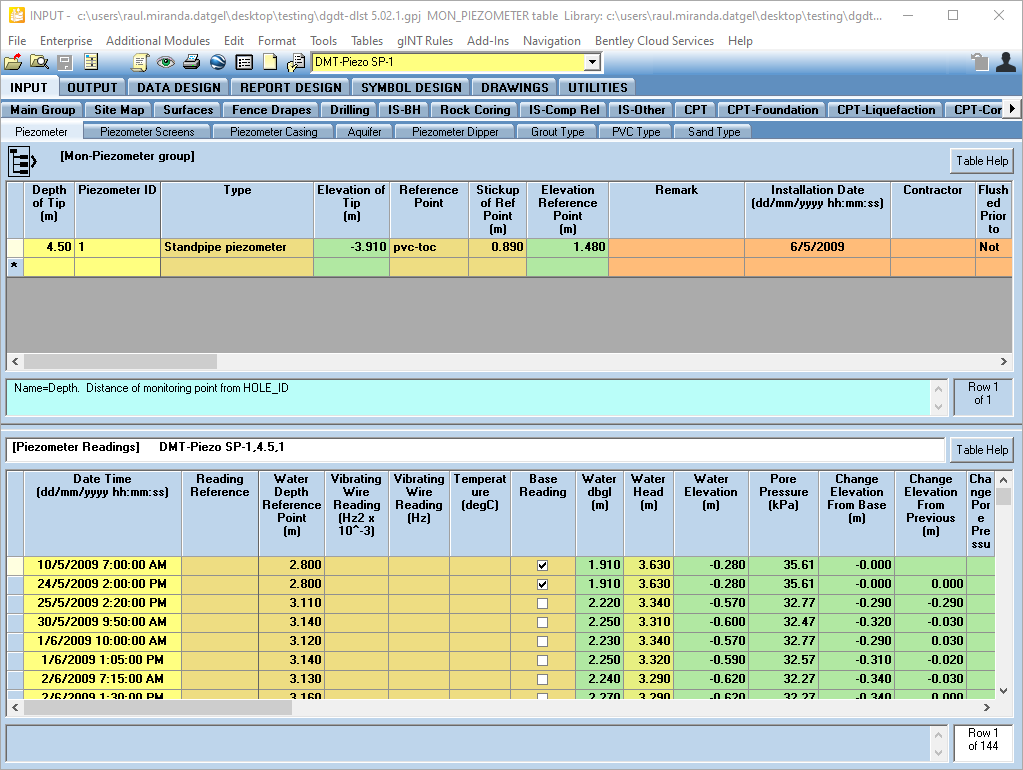
A procedure about how to enter the piezometer data into the database is detailed in the Monitoring Tool User Guide.
Log reports that present piezometer data include:
- IS AU BOREHOLE CONTAM 1
- IS AU HYBRID BOREHOLE 1
- IS AU PIEZOMETER INSTALLATION 2
- IS NZ BOREHOLE CONTAM 1
- IS NZ DRILLHOLE 1
- IS NZ DRILLHOLE 2
Selected lab results
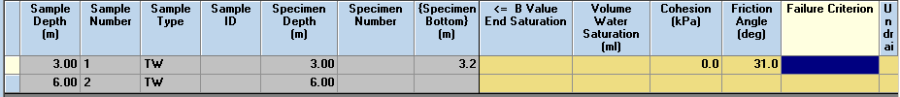
Make Specimen records
First create specimen table records – this is the bottom half of the Sample tab:
- Go to the SAMPLE tab
- On the top half of the screen click on the Depth = 6 m row
- Then on the bottom half of the screen enter 6 in the Specimen_Depth box. You may optionally enter a value in Specimen_Number
- On the top half of the screen click on the Depth = 3 m row
- Then on the bottom half of the screen enter 3 in the Specimen_Depth box. You may optionally enter a value in Specimen_Number
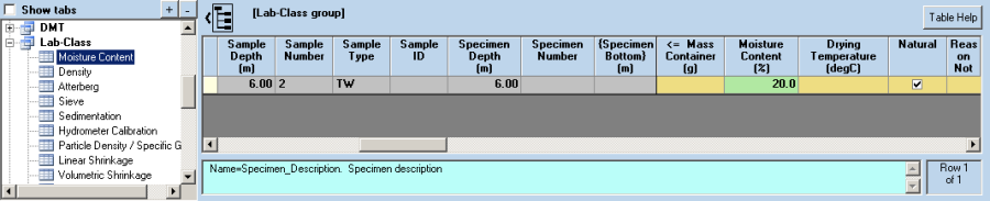
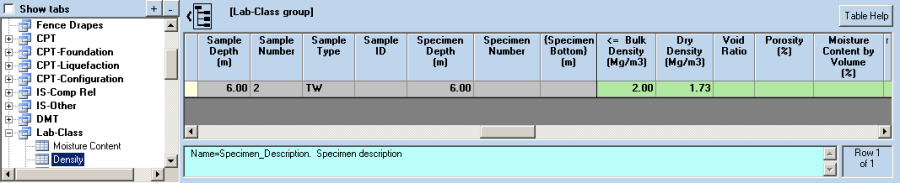
Enter Moisture Content Data
Enter Density Data
Enter Atterberg Data
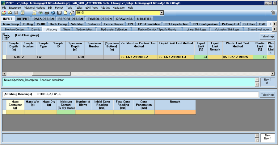
- PI and LI are calculated.
Enter Sieve Data
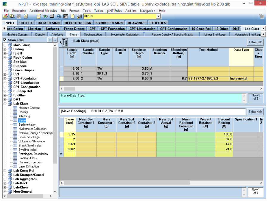
- Hydrometer results can also be entered on the Sedimentation tables
- Ensure you have made a specimen at 3.00 m before continuing.
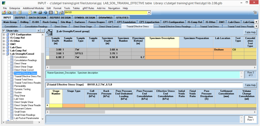
Enter Triaxial Effective Stress Data
Lab Data Entry Add-In
The Lab Data Entry feature provides the user with an option to efficiently enter and edit multiple lab results in one table interface. The procedure is as follows:
- Navigate to INPUT | Lab-General | Lab Data Entry.
- Select the desired PointID.
- Call the command, Add-Ins > Datgel DGD Tool > Pre-populate Lab Data Entry Table. This causes all existing lab data within the scope of the table to display.
- You can now complete any of these activities:
- Enter/edit data on existing records.
- Create new records and enter data. Select a Sample and enter a value for Specimen_Depth and optionally Specimen_Number.
- Delete a record by checking the delete check box.
- When the table saves a message box displays, enabling you to choose whether to update, discard, or return to the grid continue editing.
Graphical Data Input
Graphical Data Input (GDI) allows you to edit data and then instantly see the change on an interactive log report. Data entry using this interface is not as fast as Grid Input, but is ideal for data entry in the field on a tablet device, for new gINT database users who are not familiar with the fields, or when reviewing and making minor changes to data.
Click ![]() :
:
- To avoid a defect, click on the log report to make the grid window display, before using a zoom command.
- Change reports by selecting File > Select reports for Input
- Change PointID: Click anywhere on the page, and click the Select button.
- Make a new PointID: Click anywhere on the page, and click the New button.
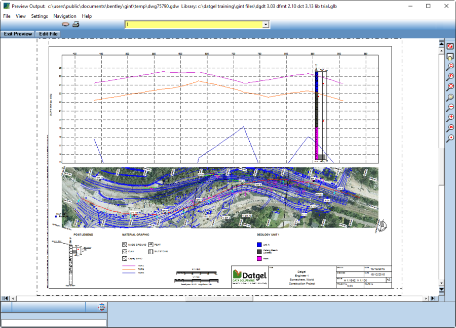
Preview from INPUT
A fast way to preview reports while entering data is to use File > Print > Preview, or the toolbar icon ![]() . You are prompted to assign a report to the table if one is not already assigned. The assigned report can be changed on the table properties form, launched by the toolbar icon
. You are prompted to assign a report to the table if one is not already assigned. The assigned report can be changed on the table properties form, launched by the toolbar icon ![]() .
.
Formatting
Format Menu
Try out some of the Format menu commands to create:
<<CLR!16711680,Very Light Blue>><<DMK!BETA LC>><<G>>=<<G>>5°<<CLR!-1>>
2<<G>>m<<SUP>>2<<SUP>>
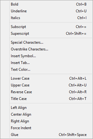
Change the text case in the Description field, double-click on the text and highlight a word or phrase. Select Format > Upper Case and notice that all of the selected words are now in upper case letters.
Interface changes
- Modifying Field Properties
- Modifying Table Properties
- Column width
- Column Order
- Row Height
- Table order
- Group order
- Assigning a table to a group can only be done in DATA DESIGN | Project Database
- Adding Fields and Tables
Input tools
- Short cut keys and scanning through records
- Text Macros
- Spell check
- View Entire Table
- Edit Entire Table
- Point Sort Field
- Comparing Databases
Replicating a Point
Use this feature to copy the currently selected PointID and all of its dependent.
- Click on the Point tab and select Tools > Replicate Point. You see the Replicate Current Point and Dependent Data dialog box:
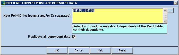
- Type BH102, BH103 in the text box to copy the current Point. The Point IDs can be separated with commas and/or carriage returns.
- When you click OK, all your new points will be defined with the common data. You can apply data changes to each PointID.
Importing/Exporting Data
gINT can interop with a wide range of file formats. These commands are located in the File menu.
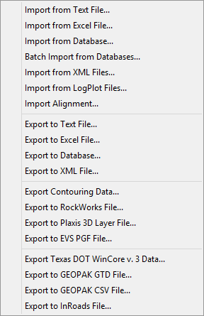
Exporting Data
Now export some data to Excel.
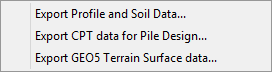
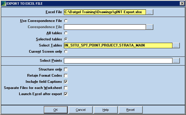
- Select the File > Import/Export > Export to Excel File menu option. You see a dialog box with specific import options.
- Click the browse
 button to the right of the Excel File text field to specify a path to a new Excel file. Call the new file "gINT Export". Check Selected tables and select the four tables in the screen shot, check Include field Captions, check Launch Excel after export and click OK to start the export.
 - At the end of the export process, any messages and errors are written to an export log. Click OK to close the window, and an Excel window will open.
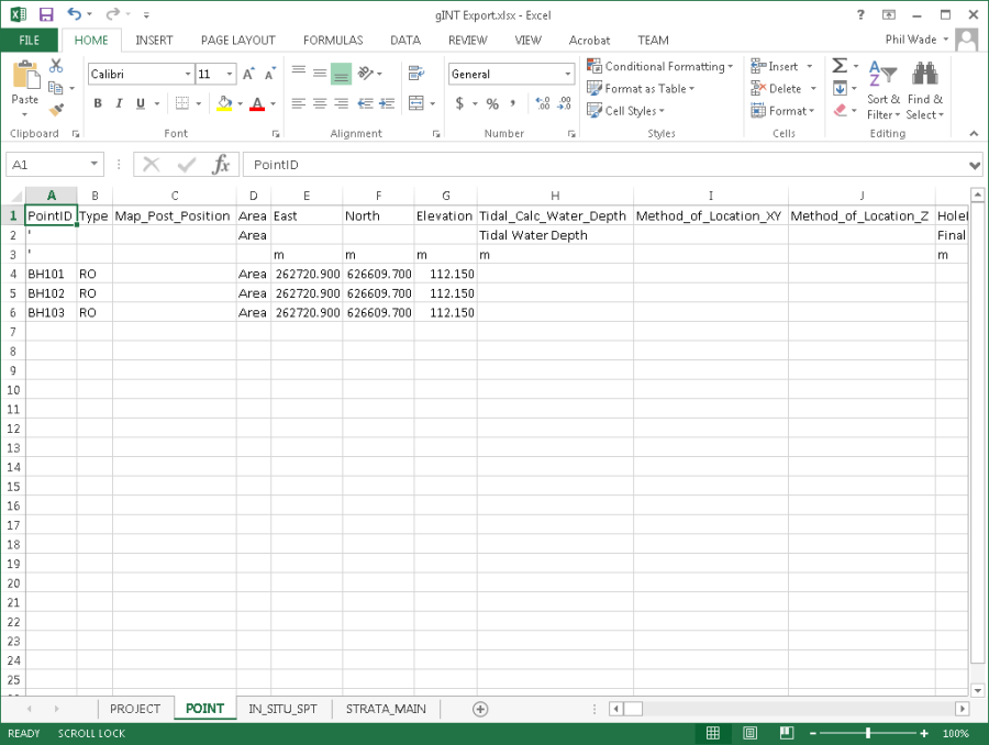
Every table in gINT is stored in a separate spreadsheet in Excel. The spreadsheets are accessible by clicking on the tabs along the bottom of the Excel screen. The first row of the spreadsheet contains the field names of the table, the second row contains the captions and units of the field, and the following rows contain the field data.
Importing Data
gINT accommodates importing data from several file formats. Common to all these import commands are two text field options, Correspondence File and Overwrite Options.
The Correspondence File field allows the program to read a gINT Correspondence File during import to map a differing file structure to the target gINT project database.
The Overwrite Option field controls how the program will deal with data that are in both the current database and the external file.
The options are:
- Never - add records who's Keys do not exist in the current database. Existing records will not be changed in any way. All options share this behaviour for new records.
- Empty fields - Writes data from the source only if the corresponding field in the target is empty.
- Named fields - Writes data from a field named in the source wherever a matching field exists in the target, overwriting any contents of the target field. Note that if a field is blank in the source it will overwrite any contents in the target field and leave it blank.
- Records - Erases each target record matched by a source record (same key) and writes the data from the source. Any records in the target that do not have corresponding records in the source will not be affected by the import.
- Data sets - Replaces entire sets of data; the resulting data set will contain only data from the source file. A "Data Set" is defined by the Keyset of the parent table. For example in a table with the PointID, Depth Keyset a Data Set is all records with a particular PointID value, while for a PointID, Depth, Reading table a Data Set is all records that share a PointID and Depth.
With the data imported to the POINT table, there is no parent table and this option acts like the Records option, that is, all the data in the POINT table will not be deleted with this option. Only the records in the target that match those in the source will be overwritten by the source data. Any records in the target that do not have corresponding records in the source will not be affected by the import.
To demonstrate the Overwrite options, modify the data in the Excel file you created previously, and import it back into the gINT database.
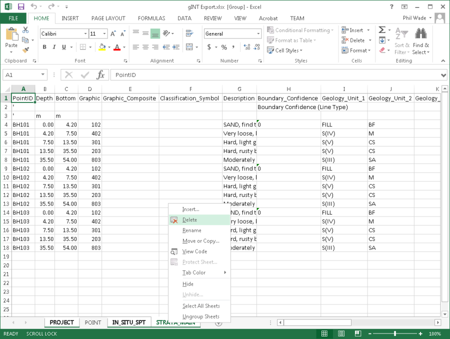
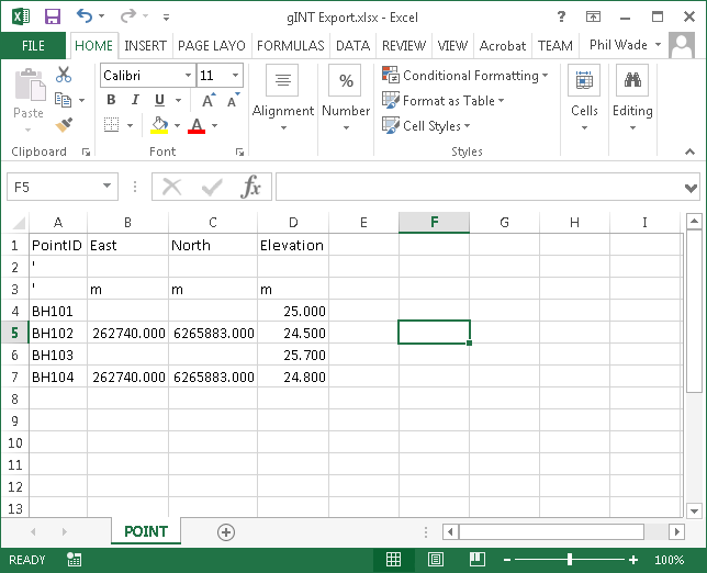
- In the Excel screen, delete all other tabs except for the POINT tab. Right click on a tab to bring up a menu, and select delete to delete a tab. Press the delete button when prompted with a message box.
- In the POINT tab, delete all the columns except for PointID, Elevation, North and East.
- Enter a new record, BH104 on the next blank row. Change the values in East, North and Elevation columns for each PointID so that they are different to each other. Leave a few values blank. The Excel spreadsheet should now look like the following screenshot.
- Save the Excel file, minimise Excel, and return to the gINT screen. Go to the Borehole tab and delete the North value for the borehole BH101, the East and North values for BH102 and the Surface Elevation, East and North values for BH103.
- Click the File > Import/Export > Import from Excel File menu option to bring up the following dialog box.
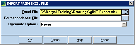
- Click the browse button to the right of the Excel File text field and select the Excel file that you have been working on. Select Never in the Overwrite Options text field and click OK.
You will see that in the import log that 0 records were imported and the records were not writable. In the Borehole table, there should not have been any changes to the existing records. This is because the Never option will not write to existing records. You will also notice that BH104 was not imported because it is missing a value in the key field HoleDepth. - Click the File > Import/Export > Import from Excel File menu option to bring up the Excel Import dialog window again. This time, select Empty Fields in the Overwrite Options text field, and click OK.
This time, you will see that the 3 Records have been added or updated. In the Borehole table, the empty East, North and Surface Elevation records will have been filled with the values in the Excel file. This option is useful if you have left the East, North and Elevation Value blank at the time of data entry, and you wish to enter these values at a later time. You will also notice that BH104 was not imported again because it is missing a value in the key field HoleDepth. - Go back to the Excel screen and enter different values for East, North and Elevation columns for all the records.
- Go to the gINT screen, and click the File > Import/Export > Import from Excel File menu option to bring up the Excel Import dialog window. This time, select Named fields (Fields not named are ignored) in the Overwrite Options text field, and click OK.
This time, you will see that 3 records have been imported. In the Borehole tab, you will see that the data in the gINT screen has been overwritten by the data in the Excel file. This option is useful if you wish to replace the existing East, North and Elevation values with more accurate values that were obtained at a later time. You will also notice that BH104 was not imported again.
Output Part 1 - Logs
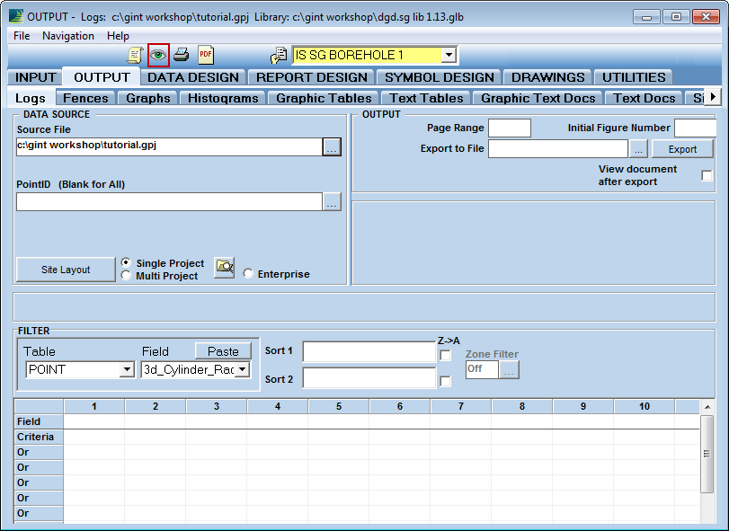
Preview all PointIDs with IS SG BOREHOLE 1
Preview Piezometer Log
- Select log report from object selector: IS AU PIEZOMETER INSTALLATION 2
- Select one PointID using the browse button
- Select preview
Open a new data source project
Click in the Source File …, and open the file dgdt #.##.gpj.
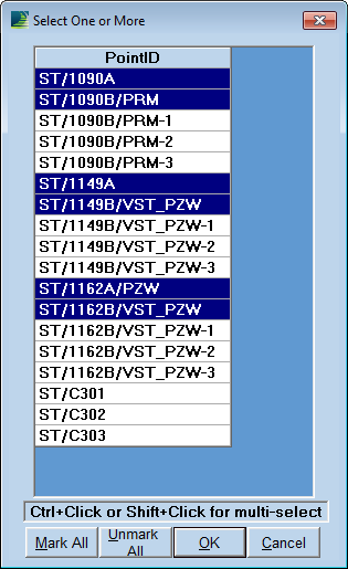
PDF a log report for multiple PointIDs with child bookmarks
- Click on the PointID… button, and using the Ctrl key, select the indicated 6 PointIDs.
- Click the PDF icon, and name a file.
- Check View document after export
- Click the Bookmark path … button
- Right click the text ROOT, and select insert child. Name item Logs
- Click on Child Bookmarks, and click OK
- Click Export
gIDraw
This is gINT's drawing interface, and is used throughout the program by users and developers.
Drawings and Layers
The object selector drop-down list, yellow list in top centre of the screen, displays the name of the current drawing. A gINT drawing file (*.gdw) may have many pages.
The Layer drop-down box in the top right of the screen displays the current layer of the drawing. If desired, you can group your entities into layers, creating an overlay in your drawing. The colour you set in the layer sets the colour of the entities at design time, but does not affect the colour at output time.

Click the Layer Properties ![]() icon to view the properties of the drawing layers:
icon to view the properties of the drawing layers:
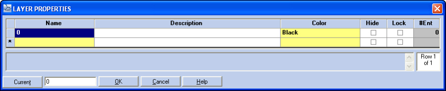
Layers are commonly used to organize entities. For example, you could place all your text entities on one layer, all your polylines on another, and so on. Or you might organize the drawing in sections with the header in one layer, the body in another and the footer in a third.
For further study on layers, select the Help > Contents > Commands > Reports > Layers topic.
The Drawing Area
In page-based gIDraw applications, you will see a page outline, or frame, similar to the following:
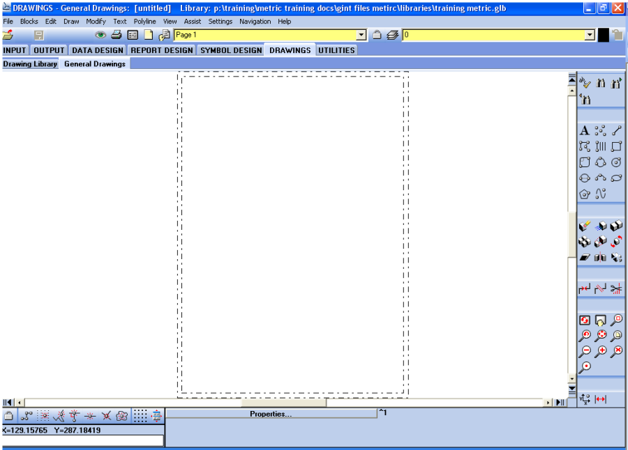
The outermost rectangle is the physical page boundaries and the next one in is the printable area for the printer associated with the drawing. The innermost rectangle corresponds to the margins that you define. By default, the margins are the "0,0" location of the X,Y coordinates, but they can be changed.
The lower right corner contains the scroll buttons to move a specified percentage of the screen height and width. If you hover over the arrow, tooltip text displays the percentage and direction the screen will move.
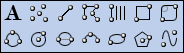
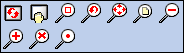
The Toolbox
The gIDraw toolbox shows some, but not all, of the commands that are available from the Drawing application menus. You can move the position of the toolbox using the Toolbox Position ![]() icon.
icon.
| Name | Command |
|---|---|
| Edit |
|
| Draw |
|
| Modify |
|
| Polyline |
|
| View |
|
| Assist |
|
| Settings/Snaps |
|
Command/Coordinate Textbox
The command text box in the lower left corner of the interface is where you enter drawing commands or your X and Y coordinates. You do not need to place your cursor in the box to enter characters; as soon as you start typing, the field is automatically populated with your entry.
![]()
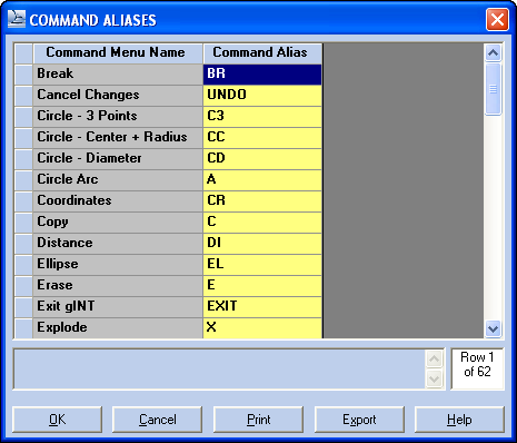
To view the command abbreviations, select the Settings > Commandline Aliases menu option. You can edit any of these command aliases and enter your own commands:
Command Panels
The bottom portion of the interface is divided into two separate panels. What is displayed here changes, depending on what you are doing in the application. If there is no command in effect, the last eight commands are displayed:

You can use a shortcut to access these commands. If you press CTRL+3, using the example above, you would activate the Select Entities command.
If you are in the middle of a multiple-step command, the middle panel displays the command that you executed and prompts you for the next step in the command and the panel to the right contains additional options for the command:

The shortcut for the Erase command is the "E" key or the DELETE key on your keyboard.
Context Menus
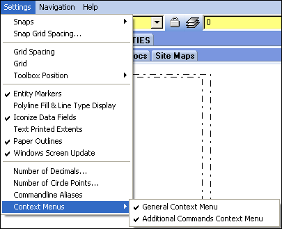
In gIDraw, the role of the right mouse button is to give you access to the context menus in gINT. By default the context menus are turned on, but you can turn them off by selecting the Settings > Context Menus option and un-checking one or both menu options.
When you right-click on your mouse with the General Context Menu turned on, the menu repeats whatever command you are working on. It also contains the Navigation, Snaps, Save and Cancel Changes options.
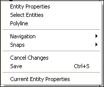
If you are in the middle of a command, accessing the context menu displays the command options, such as Erase, Move, Copy, and so on.
If context menus are turned off and there is no command in effect, when you right-click, the program executes the last command. If you are in the middle of a command, the result is the same as pressing the ENTER key.
Navigation and Zooming on a Drawing
The View tool bar contains most of the commands for navigation and zooming on a drawing. Scroll bars are located on the bottom and right of the drawing window.
| Refresh drawing |
|

Try each of the commands.
Drawing a Polyline
To draw a polyline, you can use the Polyline ![]() toolbox button, select the Draw > Points and Lines > Polyline menu option, press CTRL+L, or type PL in the command textbox. If you recently created a polyline you could select it from the list of prior commands.
toolbox button, select the Draw > Points and Lines > Polyline menu option, press CTRL+L, or type PL in the command textbox. If you recently created a polyline you could select it from the list of prior commands.
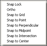
Using Snaps
When drawing polylines, you can use the snap options to place your polylines on distinct features of entities. If you click near one of the features, and use a snap option, the program "snaps" to that feature.
The Snap to Midpoint ![]() , Snap to Intersection
, Snap to Intersection ![]() , and Snap to Perpendicular
, and Snap to Perpendicular ![]() commands only apply to polylines and pseudo-polylines (the structure lines). To draw a polyline around the inner margin box on our drawing, we are going to use the Snap to Point and Snap to Perpendicular commands.
commands only apply to polylines and pseudo-polylines (the structure lines). To draw a polyline around the inner margin box on our drawing, we are going to use the Snap to Point and Snap to Perpendicular commands.
Click the Polyline ![]() toolbox button.
toolbox button.
Click the Snap to Point ![]() command and click on the lower left corner of the inside dotted frame.
command and click on the lower left corner of the inside dotted frame.
Click the Snap to Perpendicular ![]() command and click the upper right corner of the frame. gINT draws a straight line across the bottom of the frame.
command and click the upper right corner of the frame. gINT draws a straight line across the bottom of the frame.
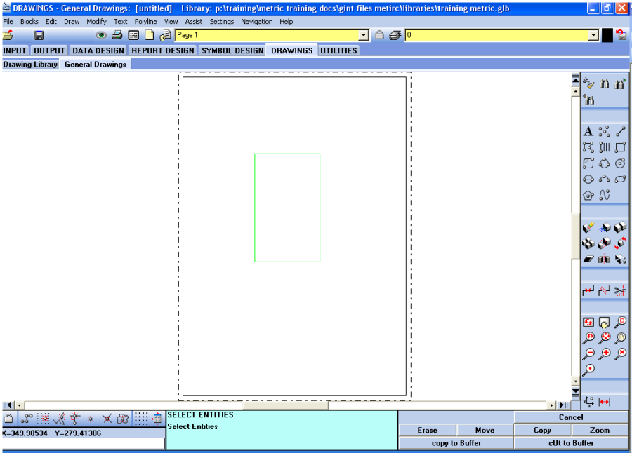
Repeat this process until all four sides of the frame are drawn and then click OK. When you are finished, your screen should look similar to the following:
To quickly erase this polyline, select the Edit > Undo Last Command menu option, press CTRL+Z, or select the entity and click the Delete key or the Erase button. There are two levels of undo; the first is undoing the last command, and the second is the Cancel Changes ![]() button, which undoes any changes made since the last time you saved your work.
button, which undoes any changes made since the last time you saved your work.
Now we can redraw the polyline using the Snap Lock ![]() command.
command.
Erase your polyline and re-select the Polyline command.
Instead of clicking on a snap command several times to draw the rectangle, we can use the Snap Lock command to repeat the same snap mode without having to re-click it each time. You can also use the SHIFT key to display the snaps menu commands.
After clicking the Polyline command, press and hold the SHIFT key and right-click your mouse. You see the following context menu:
Another way to shorten your movements is instead of using the command buttons on the lower right panel (such as Close, OK, and Cancel), when you are ready to complete a command, you can press the ENTER key, or to cancel you can press ESC. You can also press the first uppercase letter of a command to execute it. For example, if you want to close a polyline, you can type "C" on your keyboard.
You can also use the rectangle ![]() toolbox icon and the snap options to create the same polyline we did earlier. gINT does not have true circles, rectangles, arcs or ellipses. These shapes are created using polylines, which gives you more flexibility when it comes to editing.
toolbox icon and the snap options to create the same polyline we did earlier. gINT does not have true circles, rectangles, arcs or ellipses. These shapes are created using polylines, which gives you more flexibility when it comes to editing.
Draw a polyline at 0,0 by typing the coordinates in the command text box and pressing ENTER.
To offset a line from the current point, use the @ symbol and enter the new coordinates of the line. For example, if you wanted the next point of a line to be 20 mm to the right and 40 mm up from the last point, you would enter "@20,40". You can use a negative number to move the line down.
To change the angle on a point, you use polar points. You would enter the @ symbol, the length the less than symbol (<) and the degrees.
To draw a polyline starting at "50,50" that is 20 mm long at an angle of 45 degrees:
- Click the line icon, and type the initial coordinates "50,50" then click the ENTER key.
- Type "@20<45" then click the ENTER key.
To draw a circle with a set radius:
- Click the "Circle - Centre + Radius" icon, and enter the centre coordinates "50,50" then click the ENTER key.
- Type the radius preceded by @, "@20", then click the ENTER key.
To check the distance of a line, use the Assist Distance menu command or click the Distance ![]() toolbox button. When you measure the distance of a line, you see a dialog box similar to the following:
toolbox button. When you measure the distance of a line, you see a dialog box similar to the following:
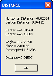
Click OK to close the dialog box. If you use the Assist Line Distance menu option, it will give you the distance of the polyline segment that you are in.
The Grid ![]() button on the Settings toolbox allows you to place a grid on your drawing area background. In the Grid Spacing dialog box, enter a number for spacing the grid points:
button on the Settings toolbox allows you to place a grid on your drawing area background. In the Grid Spacing dialog box, enter a number for spacing the grid points:
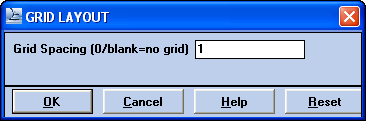
Click OK to view the grid on the workspace.
Selecting Entities
Selecting entities works the same way in gIDraw as it does in most CAD programs. In gINT, when you select an entity, it changes colour to indicate that it is selected.
You can select numerous entities by clicking on the mouse and dragging across the entities. If you go from left to right, you are specifying a non-crossing window and only the entities that are totally enclosed within the window are selected. A crossing window, which is right to left, will select any entity that is enclosed within the window or that crosses the window.
Copy and Move
- Select the circle, by clicking on the line. It will turn green
- Select the Copy button in the bottom right of the screen
- Select snap to Centre
- Click on the circle polyline
- Select Snap to Grid
- Click on the page to the right of the circle location, the copy of the circle will appear here
Move is similar.
Copy and Cut to Buffer
These copy or move entities between pages. This can be any drawing page in the current instance of gINT. Similar to the Copy example, but this time click on Copy to Buffer or Cut to Buffer
Polyline Properties
- Background fill, use this for solid
- Fill, use this for non solid fills like material graphics
- Line type, colour and thickness
Text Entity
- Click on the A icon in the tool bar
- Enter something in the Text Expression
- Set Height to a number between 1.5 and 4
- Print Opaque will place a white box behind the text, good for when you place the text on a filled polygon
- Click OK, then click within a filled polygon, where you you want the text placed.
General Commands
The majority of commands in gINT are verb-noun commands. This is when you tell the program what you want to do and on what you want to act. For example, if you want to erase a polyline or draw a circle. There are limited noun-verb commands where you first tell the program what you want to act on, and then you are given a choice of commands that you can perform on the selected entity.
Output – Part 2
Fence Exercise 1
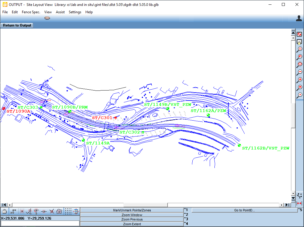
Select OUTPUT | Fences
- Click Site Layout
- Use Fence Spec. > Draw baseline
- Zoom in and use View > Go To PointID with PointID ST/109A, until you can see the data below
- Click some boreholes to select them for use on the fence
- Click on Return to Output
- Set scales, 1 = 1:1000, 30 = 1:30000, 0.1 = 1:100
- Click preview

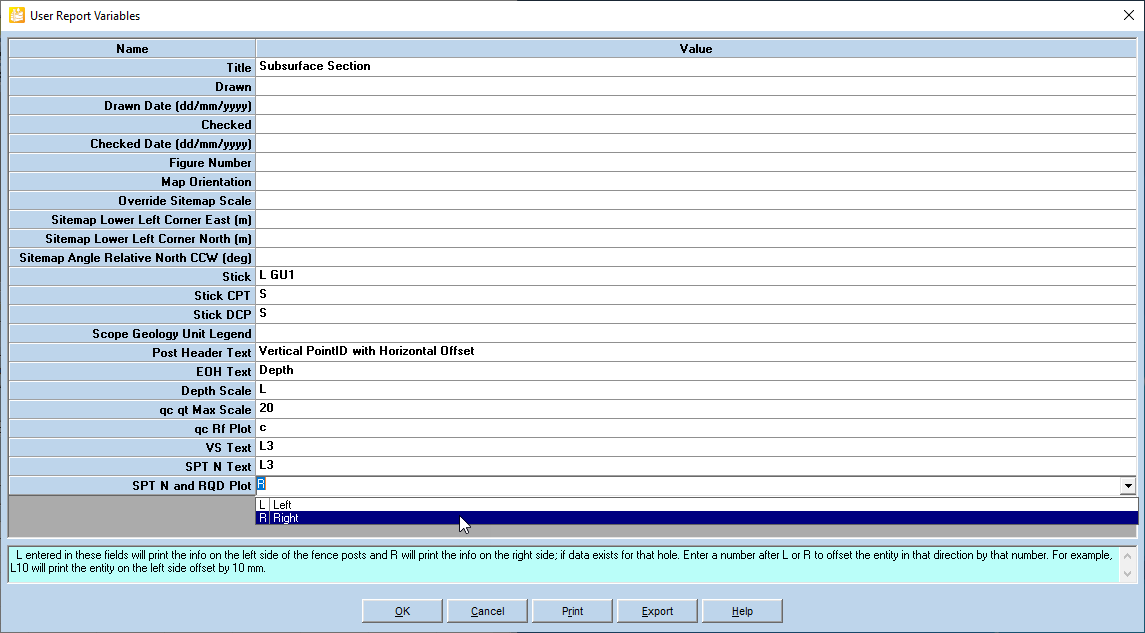
- Configure the User Report Variables as desired
- Click OK.
Fence Exercise 2
Select the INPUT application.
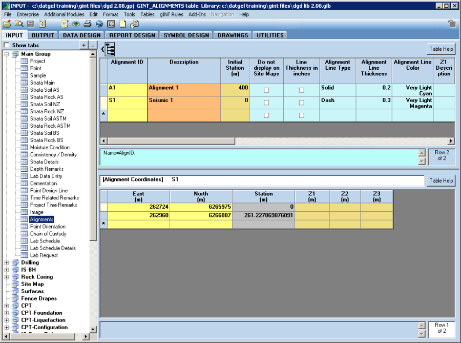
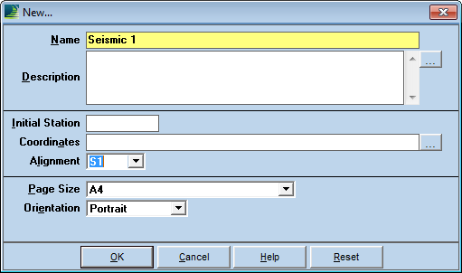
Create Alignment
Create alignment S1, and configure A1
Land XML Alignment
- Select the INPUT | Alignments.
- Select File > Import/Export >Import Alignment…, and select C:\Datgel Training \auxiliary files\Alignment 1.xml
Import DXF layout map in INPUT Site Map Application
- Select INPUT | Site Map
- Select File > Import/Export > Import DXF Import…, and select C:\Datgel Training\auxiliary files\site map dgdt.dxf
ECW File link in INPUT Site Map Application
- Select INPUT | Site Map
- Select File > Import/Export > Import Geocoded Photo…, and select C:\Datgel Training\auxiliary files\Blue Mountains.ecw
Alignment in INPUT Site Map Application
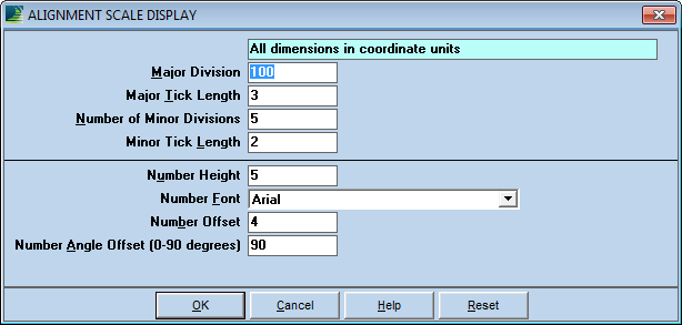
Set Site Map > Alignment Scale Display
Fence Drape
- Enable Additional Modules > Fence Drape Support.
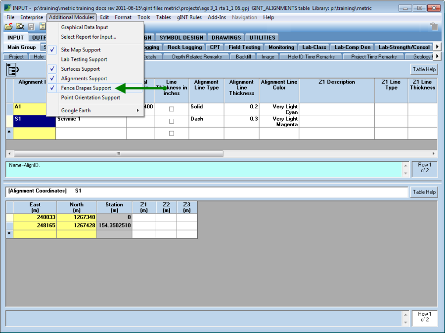
- Click the Fence Drape tab (on the far right of the table group tabs).
- Click the new icon.
- Configure the form, and click OK.
- File > Import/Export > DXF Import…. Select C:\Datgel Training\auxiliary files\SL 1.dxf
- Select the text Seismic refraction DXF output test by clicking to the bottom left of the text, then clicking to the top right of the text. Then, press the Delete button.
Output
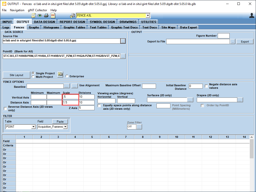
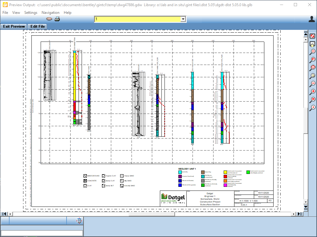
Now move to OUTPUT | Fences. Configure:
- Report: FENCE A3L or FENCE MAP A3L
- Use Alignment: A1
- Baseline offset: 20
- Drapes: check Seismic 1, set Text Scale 0-100 = 0
- Preview
- Configure User Report Variables
- Click on Edit File, and provide a file name for the *.GDW gINT drawing file.
- Add annotations and filled polygons
- Export to DGN
- Select File > Import/Export > Export DGN...
- Set the seed file: C:\Users\Public\Documents\Bentley\gINTCL\seed\seed2d_millimeters.dgn
- Check Launch MicroStation after export
- Click OK
Graphs
- Preview the following reports
- A IS SPT N VS RL BY UNIT
- A L CS ATTERBERG BY SPECIMEN
- A L CS MC VS DEPTH BY PTID
- A L CS PSD 10 PER PAGE SUMMARY - select about 20 specimens
A L S SU UU VS RL BY UNIT
- Configure the range filter, in the Criteria row select Like from the drop down, the type <spacebar>O*
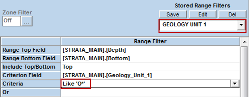
- Preview the same reports again
Other reports
Now preview Histogram, Graphic Table, Text Table, Graphic Text Document, Text Document, and Site Map reports.
Further Output Options
- Filter
- Sort
- Scripts
AGS Format
Export AGS Format data
- Navigate to INPUT
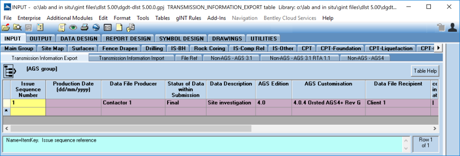
- Set the fields AGS_Edition and AGS_Customisation, on the AGS | Transmission_Information_Export table. For example, 3.1, 3.1 RTA 1.1 or 4.0 in the AGS_Edition (not 4.0.3 since some competing software can't handle it). If you are exporting ASG4 select an AGS Customisation in the drop-down list.
Select File > AGS Files > Export to AGS File…
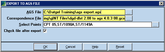
- Set the AGS File to make.
- Browse to the relevant Correspondence File for the version of AGS you need to export.
- For AGS 3.1: dgdt-dlst 4.## to ags 3.1 ##.gcx
- For AGS 3.1 RTA 1.1: dgdt-dlst 4.## to ags 3.1 rta 1.1 ##.gcx
- For AGS4: dgdt-dlst 4.## to ags 4.0.3 ##.gcx
- Select PointID or leave it blank for all, and click OK.
- Review the export log for problems, save the text log file for future reference, click OK.
On the checker form, click View Report, and name a file to save it as. The checker report will now display in a text editor.
FYI are not generally a concern, if you find errors you should investigate the issue, and if needed contact Datgel for advice.
Open the AGS file in a text editor (such as Notepad++) and review the data and file layout/
Import AGS Format data
- Navigate to INPUT, and open the target project, or make a new project
- Select File > AGS Files > Import to AGS File…
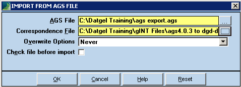
- Select the AGS File to import.
- Browse to the relevant Correspondence File for the version of AGS you need to import.
- For AGS 3.1: ags 3.1 to dgdt-dlst 4.## ##.gci
- For AGS 3.1 RTA 1.1: ags 3.1 rta 1.1 to dgdt-dlst 4.## ##.gci
- For AGS4: ags 4.0.3 to dgd-dlst 4.## 07.gci
- Configure the Overwrite Option, normally Never is appropriate.
- If you have not previously checked the AGS file, it is a good idea to do so before import, to do so check the box.
- Click OK.
- If you checked the AGS file, on the checker form, click View Report, and name a file to save it as. The checker report will now display in a text editor. FYI are not generally a concern. If there are errors, you could send the file to the data generator and request they correct the problems. If you wish to proceed with the import, click OK on the form now visible in gINT.
- Review the import log for problems, click OK. You may like to save this to a text file for future reference.
- Review the data imported. Look for data completeness and correct units etc.
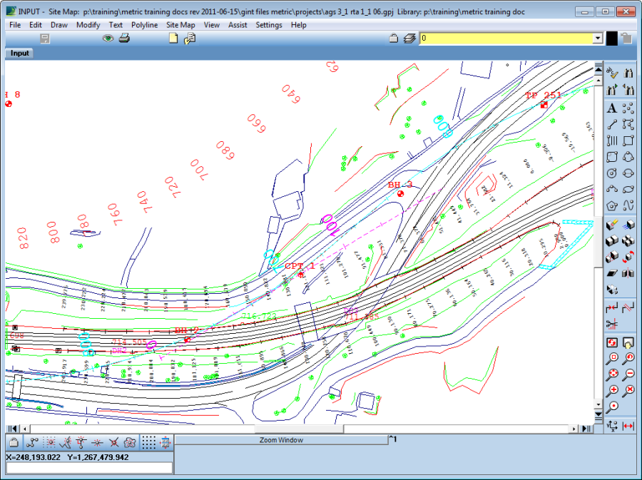
Site Map
- Using Site Maps as a Project GIS
- View and edit Point table data
- View project data
- Moving exiting PointIDs
- Laying out Drilling Programs with Site Maps
- Make a Zone
- Use zone filter with Site Map Report
Utilities
In this section, we will discuss the UTILITIES application group and the purpose of each of the applications. The UTILITIES applications are primarily program maintenance applications, designed to help streamline some of the database processes in gINT.
Repair/Compact Databases
Occasionally, databases get corrupted. If that happens in gINT, you can use this application to repair the file. In addition, this utility removes deleted records. Like most databases, the records are not actually deleted in the Microsoft ACCESS files that gINT uses, they are marked as deleted and not shown.
We recommend using this utility on your library file once a month to repair and compact the file. It is a good idea to do the same for large, long-running projects. When you click the Repair/Compact Databases application tab, you see the following dialog box:
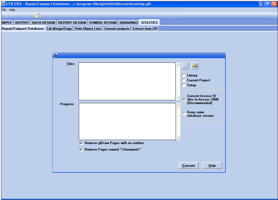
To repair/compact a database, you would enter the database name in the Files text box, or click the browse ![]() button to select the file. Instead of browsing for a file, you can select one of the following options:
button to select the file. Instead of browsing for a file, you can select one of the following options:
- Library to repair/compact the current library.
- Current Project to repair/compact the current project database.
- Setup to repair/compact your SETUP.GSH file.
After choosing your files, you would select from one of the following options:
- Convert Access 97 files to Access 2000 (default) to convert the files to Access 2000. ACCESS 2000 handles the transition between double and single byte environments better than ACCESS '97. gINT versions 5 and 6 work equally well with ACCESS '97, 2000, or XP version files.
- Keep same database version to keep the current version of Access and not convert the files to Access 2000.
- The Remove gIDraw Pages with no entities option removes all empty gIDraw pages, regardless of the name. The Remove Pages named ">Unnamed<" option removes all library pages. Both options apply only to library files. Click the Execute when you are ready to repair/compact the database.
For further study, select the Help > Contents > Utilities Application > Repair/Compact Databases topic.
Print Object Lists
This application allows you to batch print the entire contents of all symbol, graphic report, and drawing libraries.
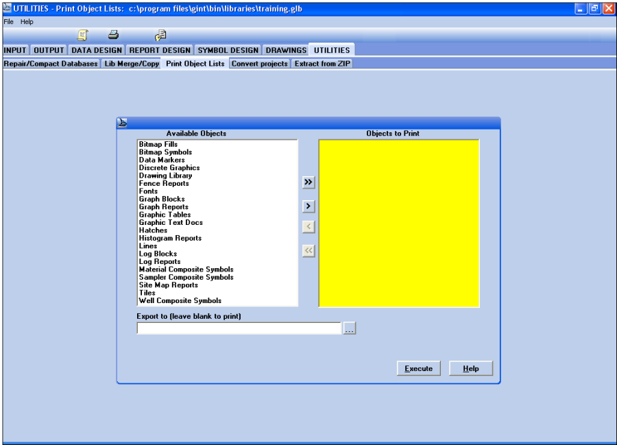
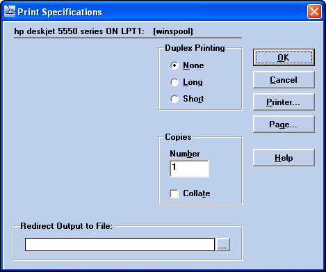
To print, just move the file(s), from the Available Objects list to the Objects to Print list using the arrow buttons and then click Execute. Select your print specifications in the dialog box that displays:
For further study, go to Help > Contents > Utilities Application > Print Object Lists
Convert Projects
Convert Projects allows you to convert existing projects to a different database structure using a data template file and an optional correspondence file. The structural changes could be minor such as a changed caption, ranging to major changes such as new tables and fields.
When you click on the Convert Projects application tab, you see a dialog box similar to the following:
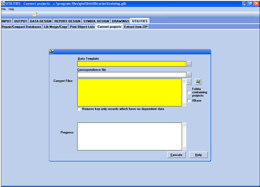
Specify the target Data Template file. This is the file that stores the structure you want to convert the projects to. The Correspondence File is used to map the old structures into the new and the lists of projects (Convert Files) are the files you wish to convert. Click Execute to convert the files. For each project file being translated, gINT will:
- Create a temporary file with the structure of the specified Data Template.
- Copy the data from the project file to the temporary file according to the mapping specified in the Correspondence File.
- Rename the original project file to <original name>.ORG in the same folder. This creates a backup file.
- Rename the temporary file to the name of the original project file <original name>.GPJ. For example, when you have converted "PROJECT1.GPJ", then "PROJECT1.GPJ" will be the new file and "PROJECT1.ORG" will be the original file.
- Remove the file name from the Source Files list and add it to the Converted Files list, appending "OK" if the conversion was successful, "Failed" if there was a fatal problem (such as not being able to open the file,) or "Cancelled" if Cancel was clicked during a conversion.
- Display a full report after all files have been converted.
If a field in a project file is not mapped to the Data Template through the Correspondence File, the data contained in that field will be lost. Do not delete the backup files until you are sure the converted projects are correct.
For further study, select Help > Contents > Utilities Application > Convert Projects
DTM to LandXML
- Select to INPUT | Additional Modules > DTM to LandXML
- Configure the following:
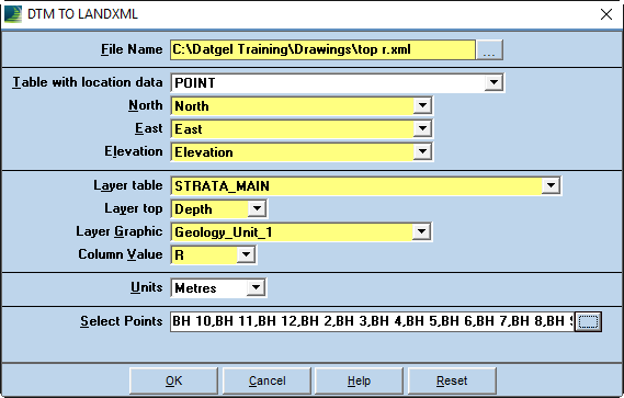
- Do similar for Top B and Top R.
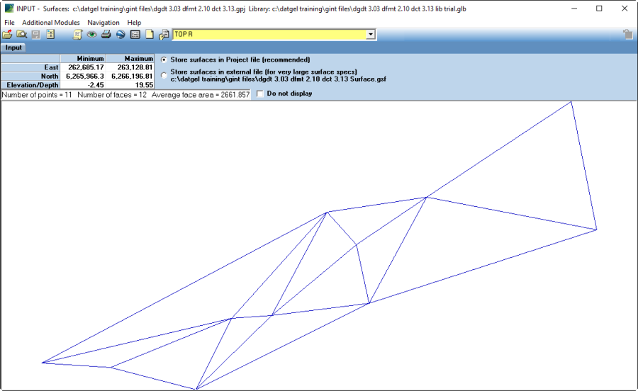
- Select INPUT | Surfaces
- Select the New icon, and Import the Top R LandXML TIN
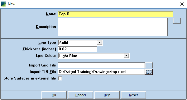
- Do similar for Top A and Top B, but use a different colour.
- Move to OUTPUT | Fences, and configure the following:
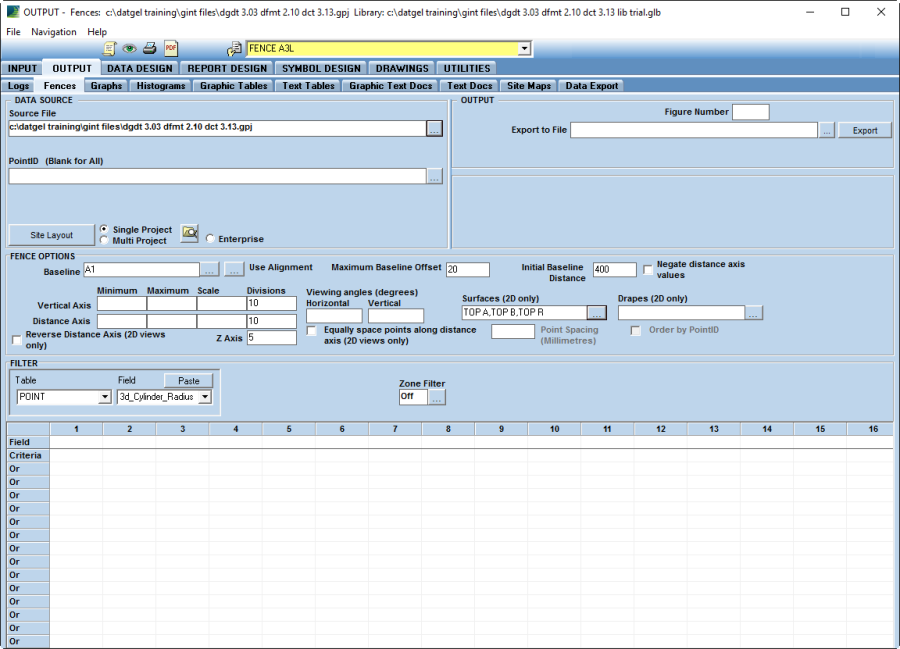
- Preview
Writing Queries
If you have some knowledge of SQL (Structured Query Language), you can create reports containing a series of commands that filter and manipulate your data at output time. Queries are created in INPUT using the Tools > Queries menu option and OUTPUT using the File > Queries menu option.
Example Query 1
select [STRATA_MAIN].[PointID], [STRATA_MAIN].[Depth], [STRATA_MAIN].[Bottom], [STRATA_MAIN].[Graphic] from [STRATA_MAIN]
Use CTRL + right mouse button on the Paste button to paste table name only.
The above will return a list of BH numbers, top depths and legend codes. Note column headers are taken from the fieldname caption. This can be printed or exported to a file (e.g. XLS).
To order the data by key fields, insert the following after the existing code. Click ‘Edit’ button to amend query.
order by [STRATA_MAIN].[PointID], [STRATA_MAIN].[Depth]
To add a filter, insert the following after the existing code. before the order by. Click ‘Edit’ button to amend query.
where [STRATA_MAIN].[Graphic] like '4*'
For multiple filters add
and [STRATA_MAIN].[Depth] < 5.0
This will return all of the depths where with a Sand legend and is above 5m depth.
To sort the list by GintPointSort, we need to join STRATA_MAIN with POINT
select [STRATA_MAIN].[PointID], [STRATA_MAIN].[Depth], [STRATA_MAIN].[Bottom], [STRATA_MAIN].[Graphic], [POINT].[GintPointSort]
from [STRATA_MAIN] inner join [POINT] on [STRATA_MAIN].[PointID] = [POINT].[PointID]
where [STRATA_MAIN].[Graphic] like '4*' and [STRATA_MAIN].[Depth] < 5.0
order by [POINT].[GintPointSort], [STRATA_MAIN].[PointID], [STRATA_MAIN].[Depth]
Example Query 2
A further example where the header is not a caption, and the use of aggregate functions:
select count(*) as [Number of Points],
sum([POINT].[HoleDepth]) as [Total length drilled]
from [POINT]
Will give a table as follows (example)
Number of Points > Total length drilled
Now make this query more complex by adding group by Hole Type
select [POINT].[Type] as [Type], count(*) as [Number of Points],
sum([POINT].[HoleDepth]) as [Total length drilled]
from [POINT]
group by [POINT].[Type]
The SQL expression is given a ‘Name’ and ‘Description’ for subsequent use.
SQL References
The following website give a good explanation of SQL: http://www.w3schools.com/sql/default.asp
For further study, go to the Help > Contents > Commands > Input > Queries topic.
Coordinate Tool in gINT Professional Plus
This allows the user to assign a coordinate system to a project, and gINT will then automatically calculate Latitude and Longitude in WGS84 for each PointID. This data in stored on two fields on the POINT table.
Say you have Latitude and Longitude data to WGS 84, and wish to calculate East and North to a particular coordinate system. Under this scenario you should enter data into POINT fields WGS84 Latitude and WGS84 Longitude, then define a coordinate system on the PROJECT table, and East and North will be calculated.
Say you wish to convert the coordinate system of a set of data. First define the source coordinate system on the PROJECT table, and the POINT fields WGS84 Latitude and WGS84 Longitude will calculate. Then delete then clear the Coordinate System field on the PROJECT table, and clear the East and North fields on the POINT table. Finally, assign the new coordinate system on the PROJECT table and the new East and North will automatically calculate.
You will also need to set the Coordinate_Unit field on the PROJECT table appropriately.
The Elevation Offset field on PROJECT is used to relate elevation datum between projects. Say one project uses LAT for near shore boreholes, another project uses AHD for onshore boreholes, and you wish to present a fence diagram using AHD using boreholes from both projects. In the near shore project, you should set the Elevation Offset field to correct offset value for the location of work, e.g. 0.524 (for Williamstown, Victoria).
gINT Professional Plus V8i (select series 2) 8.3.3 has a new feature that facilitates user defined coordinate systems created using Bentley Map. See https://www.datgel.com/gint-faq for the procedure.
Exercise to define a coordinate system
- If need be enable Coordinate fields from Tables > Coordinate Fields. This adds fields to the PROJECT and POINT tables.
- Go to POINT table, and delete and values in WGS84_Latitude and WGS84_Longitude. Delete and data for East and North where the values are not in the order of 26#### and 626####.
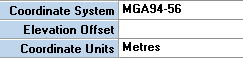
- On Project table, click on the Coordinate System browse button, and configure:
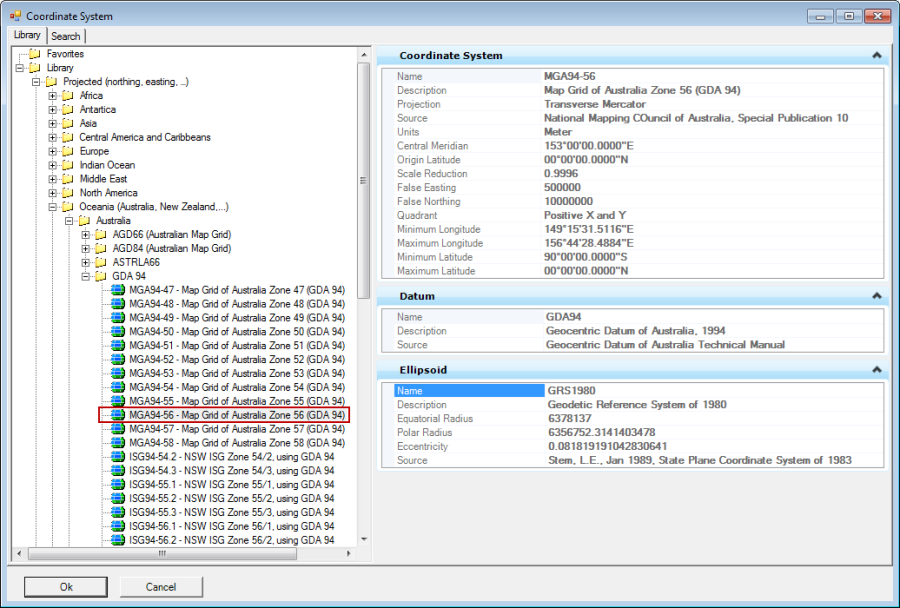
- Set Coordinate Units to Metres
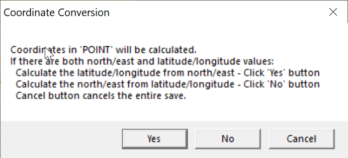
- Move to the Point table, and you will be asked what to calculate. Select Yes, to calculate Lat/Long from East/North.
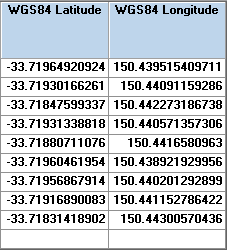
Google Earth Export
- Select Additional Modules > Google Earth > Google Earth Setup…
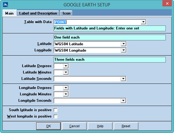
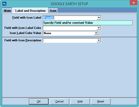
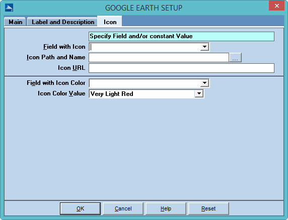
- Now select the Google Earth toolbar button
 , and configure the following.
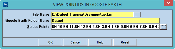
- Click OK.
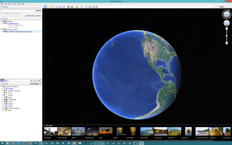
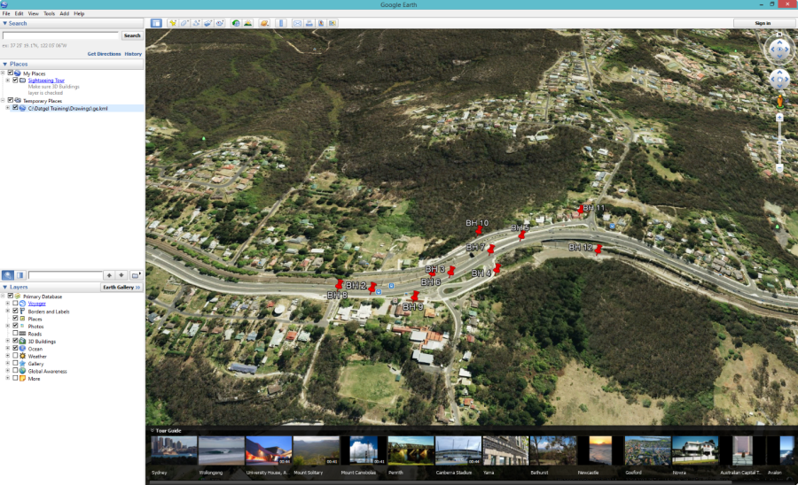
- Google Earth will now launch, and zoom into the area.
On this page