Input
Overview
The INPUT application is where project data is entered and calculated, and is the primary area where data can be imported and exported.
Make a new Microsoft Access format Project
To make a new Access format Project File:
- Select INPUT | File > New Project or the
 (new) icon > Clone Data Template…
 - Browse to the data template dgdt 4.##.gdt or your companies gdt file, and click Open
- Name the new project file, and click Save
Database Structure
The project database tables are grouped and ordered in a logical way, with borehole-related table groups first in the list, followed by in situ testing, lab testing, and then other tables.
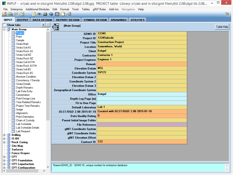
INPUT with tree and tab navigation
Logo
The logo on all reports is controlled by the field PROJECT.Office. This allows the library to be configured with multiple organisation brandings, and you can easily select the required branding.
See section Configuring Logos in the Library for further details.
Importing Pre-Existing Data from Old Project Structure
It is possible to import data from your old project structure. How easy that will be depends upon if your old structure is similar to those Datgel has developed import correspondence files for. The standard import correspondence files are:
- ags 3.1 rta 1.1 06.2 gint db to dgdt-dlst #.## ##.gci – use with database import to import a AGS RTA project database into a DGDT project database.
- gint std ags 3.1 w lab tables to dgd-dlst #.## ##.gci gci – use with database import to import a gINT standard AGS 3.1 project database into a DGDT project database.
- gint std australia to dgd-dlst #.## ##.gci gci – use with database import to import a standard Australia gINT project database into a DGDT project database.
You can use these with the following gINT features:
- UTILITIES | Convert Projects
- INPUT | File | Import/Export > Import from Database…
- INPUT | File | Import/Export > Batch Import from Database…
One can edit or make new correspondence files in DATA DESIGN | Correspondence Files. It is likely to be cheaper to get Datgel to develop this for you on a consulting basis rather than do this in house, as it is not a skill you will use on a regular basis. This is a native gINT feature, and if you require technical support you should contact your gINT Technical Support provider.
General Data Entry
The simplest way to produce your first gINT log is to use Graphical Data Input, rather than Grid Input. This can be accessed under Additional Modules > Graphical Data Input or by clicking the following icon ![]() . You can then see a representation of the log on the screen and click the data area of interest. The associated tables will popup.
. You can then see a representation of the log on the screen and click the data area of interest. The associated tables will popup.
To change the log report you are working with, go to File > Select Report for Input. To change PointID when in Graphical Data Input, double-click anywhere on the log image to bring up the grid sub form, then click Select PointID to bring up the PointID list, then select the desired PointID.
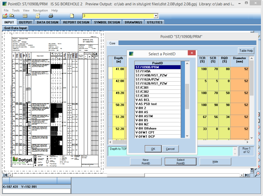
Graphical Data Input
The alternative is Grid Input which is a spreadsheet type interface. This is faster and more convenient for users with experience of the data structure. This interface is the default and can be returned to by clicking the Grid Data Input tab.
Log output option fields
Option fields exist on PROJECT, POINT, PROJECT_OPTIONS and POINT_OPTIONS.
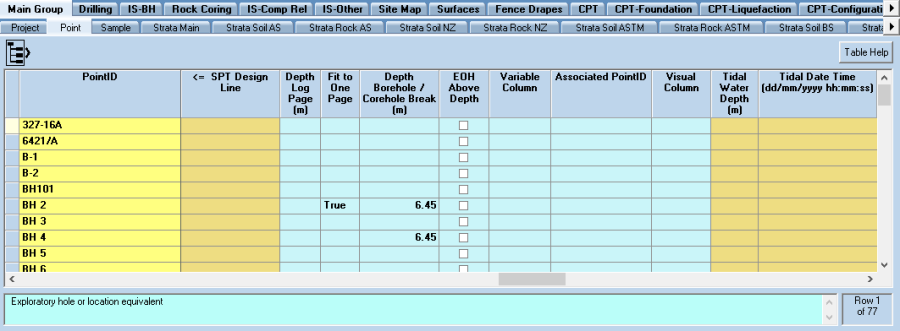
POINT table log output option fields
Metres per page
Fields Depth_Log_Page and Fit to One Page on POINT and PROJECT override report level defaults for metres per page. Applied to all log reports.
Break depth and between non cored and cored logs
POINT.Depth_Borehole / Corehole Break: Depth at which non-cored borehole stops and cored borehole begins; If the borehole contains core only then set this field to 0, if the borehole has non-core only then leave this field blank. Applies reports:
- Log | IS AU BOREHOLE 1
- Log | IS AU BOREHOLE 2
- Log | IS AU BOREHOLE 3
- Log | IS AU CORED BOREHOLE 1
- Log | IS AU CORED BOREHOLE 2
- Log | IS AU CORED BOREHOLE 3
- Log | IS NZ BOREHOLE CONTAM 1
- Log | IS NZ DRILLHOLE 1
- Log | IS NZ DRILLHOLE 2
- Log | IS UK BOREHOLE
- Log | IS UK DRILLHOLE
Display end of hole remark above depth to avoid overlaps
POINT.EOH_Above_Depth: Check if end of hole remark is to display above the hole depth. This maybe to avoid an additional page just to show a remark, or to stop text running into footer.
Optional manual override for column on right of logs
POINT.Variable_Column: Used by a limited number of logs to define if DCP, Piezometer or Additional Observations data will display in column on right side of log. Applies to reports:
- Log | IS AU BOREHOLE CONTAM 1
- Log | IS AU BOREHOLE 3
- Log | IS AU TEST PIT 3*
Rock Fracture Data representation on logs
POINT.Fracture_Column and PROJECT OPTIONS.Fracture_Column Used by a limited number of logs to define if Rock Fracture will display as Average Defect Spacing or Fracture Frequency. Applies to reports:
- Log | IS AU CORED BOREHOLE 1
- Log | IS AU CORED BOREHOLE 2
- Log | IS AU CORED BOREHOLE 3
SPT Data
The SPT calculation is designed to support BS, ASTM and AS methods. Note:
- If you use a test method that records three intervals, then enter the results in columns 1st, 3rd, and 5th.
- Default Penetration interval values are set on the PROJECT table in fields Default_SPT_Pen_1_3_5 and Default_SPT_Pen_2_4_6. For AS/ASTM set the former to 150 and later blank, and for BS set both to 75.
- The N_Value and Reported_Result fields both must be empty for the basic SPT calculation to take place. The N60 calculation will take place regardless as long at the N_Value is defined or calculated.
- The calculation for N_Value and Reported_Result fields have options defined on Project_Options:
- SPT_Sample_Type: Sample Type used when auto generating Sample table record for an SPT with recovery
- SPT_N_Value_Refusal: Blank for nothing, or set a number such as 50 or 100
- SPT_Reported_Result_N_value_Refusal: select from a drop down list of syntax: N=R, N>50, N>100, N=##/##mm or N not reported.
- SPT_Reported_Result_Length_Unit: Select from a lookup list of m, cm or mm
- SPT_Star_Suffix_for_Recovery: Check to populate Reported Result with N* when Recovered Length is > 0
- SPT_Wrap_Character_Length: Controls the reported result length
- Pore Pressure, Total_Stress and Effective_Stress are calculated based on the Depth and data entered in the Project_Options and Point_Options tables.
SPT Supported Test Methods
Standard | Description |
|---|---|
AS 1289.6.3.1-2004 | Determination of the penetration resistance of a soil - Standard penetration test (SPT) |
BS1377-9:1990:3.1 | Standard Penetration Test |
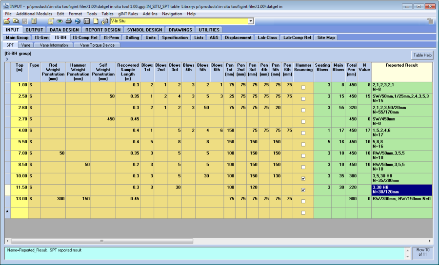
SPT Test Tables
Data Entry Procedure:
- Enter the Top depth of the test and select the Type of test undertaken.
- If you enter the Recovered_Sample_Length, a Sample table record will be created corresponding with the SPT test depth range.
- For the British Standard method:
- Enter the Self_Weight_Penetration, i.e. the penetration under the rod and hammer weight.
- Enter the blow count recorded for each increment in the applicable blows field (Blows_1st, Blows_2nd, Blows_3rd, Blows_4th, Blows_5th and Blows_6th).
- Each increment penetration field (Pen_1st, Pen_2nd, Pen_3rd, Pen_4th, Pen_5th and Pen_6th) is automatically populated with a default value of 75 mm and this can be overridden with the actual increment penetration value for each respective blow count.
- For the Australian Standard method:
- Enter the Rod_Weight_Penetration and Hammer_Weight_Penetration if applicable
- Enter the blow count recorded for each increment in the applicable blows field (Blows_1st, Blows_3rd, and Blows_5th).
- Each increment penetration field (Pen_1st, Pen_3rd, and Pen_5th) is automatically populated with a default value of 150 mm and this can be overridden with the actual increment penetration value for each respective blow count.
The Seating_Blows, Main_Blows, Total_Pen, N_Value (not calculated if the test does not reach 450mm) and Reported_Result will be automatically calculated when you change table or click save (Ctrl+S).
N Value and Reported Result must be empty for the row to calculate
- If you have entered data on the In Situ Point Options and / or In Situ Project Options tables, then the Total_Stress, Effective_Stress and C_N fields will be automatically calculated when you change table or click save (Ctrl+S).
- To calculate the N{}_{60} and (N{}_{1}){}_{60} values, see the following detailed explanation below in section Correlations.
Correlations
The primary reference for the N{}_{60} and (N{}_{1}){}_{60} calculations was Skempton (1986). The following table has been reproduced from the paper and presents the correction values used the in the N{}_{60} and (N{}_{1}){}_{60} calculations.
SPT Field Procedure Corrections (Skempton 1986)
Factor | Value | Equipment Variable |
|---|---|---|
Energy Ratio CER | 0.90 | Safety Hammer |
0.75 | Donut Hammer | |
Borehole Diameter CB | 1.00 | 65 to 115 mm |
1.05 | 150 mm | |
1.15 | 200 mm | |
Sampling Method CS | 1.00 | Standard Sampler |
1.20 | Sampler without liner | |
Rod Length CR | 1.00 | > 10 m |
0.95 | 6 to 10 m | |
0.85 | 4 to 6 m | |
0.75 | 3 to 4 m |
These correction values are each stored in the library file and; depending on the data entered into the Hammer_Type, Borehole_Diameter, Sampling_Method and Rod_Length fields; the appropriate value from the library table will be written to the corresponding C_{ER}, C_B, C_S, and C_R field and used to calculate the N{}_{60} and (N{}_{1}){}_{60} values, when you change table or click save (Ctrl+S).
The Corrected N Value (N{}_{60}) is defined as:
| \[N_{60}=\frac{C_{ER}\cdot C_B\cdot C_S\cdot C_R\cdot N}{0.6}\] |
Total Stress ({\sigma }_{vo}) is defined as:
| If\ z<{z_{\mathrm{w}}\ or\ z_{\mathrm{w}}\ is\ null\ then\ \sigma }_{vo}=z\cdot \gamma \\ If\ z\ \ge {z_{\mathrm{w}}\ then\ \sigma }_{vo}=z_{\mathrm{w}}\cdot \gamma \ +\ \left(z-z_{\mathrm{w}}\right)\cdot {\gamma }_s |
Where:
z is Top depth on the SPT table
z_{\mathrm{w}} is Groundwater_Depth on the In_Situ_Point_Options table (or In_Situ_Project_Options table if there is no value on the In_Situ_Point_Options table)
\gamma is Bulk_Unit_Weight on the In_Situ_Point_Options table (or In_Situ_Project_Options table if there is no value on the In_Situ_Point_Options table)
{\gamma }_s is Bulk_Unit_Weight_Saturated on the In_Situ_Point_Options table (or In_Situ_Project_Options table if there is no value on the In_Situ_Point_Options table)
Effective Stress (\sigma'_{vo}) is defined as:
| If\ z<{z_{\mathrm{w}}\ or\ z_{\mathrm{w}}\ is\ null\ then\ \sigma'}_{vo}={\sigma }_{vo}\\ If\ z\ \ge z_{\mathrm{w}}\ then\ {\sigma'}_{vo}={\sigma }_{vo}\ -\ \left(z-z_{w}\right){\cdot\rho }_w\cdot g |
Where:
z is Top depth on the SPT table
z_w is Groundwater_Depth on the In_Situ_Point_Options table (or In_Situ_Project_Options table if there is no value on the In_Situ_Point_Options table)
\rho_{w} is Water_Density_In_Situ on the In_Situ_Project_Options table
g is Gravity
The Overburden Correction Factor (C_N) proposed by Liao and Whitman (1986) is defined as:
| C_N\mathrm{=}{\left(\frac{\mathrm{100}}{{\mathrm{\sigma }}^{\mathrm{'}}_{\mathrm{vo}}}\right)}^{\mathrm{0.5}} |
The N Value corrected for Overburden Pressure ((N{}_{1}){}_{60}) is defined as:
| {\left(N_1\right)}_{60}\mathrm{=}{\mathrm{C}}_{\mathrm{N}}\cdot N_{60} |
Output
- Logs | IS SPT DESIGN LINE
- Many other log reports
- Graphs | A IS SPT (N1)60 VS DEPTH BY PTID
- Graphs | A IS SPT (N1)60 VS DEPTH BY UNIT
- Graphs | A IS SPT (N1)60 VS RL BY PTID
- Graphs | A IS SPT (N1)60 VS RL BY UNIT
- Graphs | A IS SPT N VS DEPTH BY PTID
- Graphs | A IS SPT N VS DEPTH BY UNIT
- Graphs | A IS SPT N VS RL BY PTID
- Graphs | A IS SPT N VS RL BY UNIT
- Graphs | A IS SPT N60 VS DEPTH BY PTID
- Graphs | A IS SPT N60 VS DEPTH BY UNIT
- Graphs | A IS SPT N60 VS RL BY PTID
- Graphs | A IS SPT N60 VS RL BY UNIT
- Histograms | A IS S SPT N
Pocket Penetrometer
There are three tables where Pocket Penetrometer (PP) can be entered:
- IS-BH | Vane PP TV - for test done in situ or in a sample when in the field
- Sample (bottom half) i.e. Specimen table - for tests done in sample in the field. This will be deprecated in future.
- Lab-Strength/Consol | Lab Pocket Penetrometer - for test done in lab, and this is not linked to log reports.
There are a two sets of fields
- UCS results, which is the number directly read from the device
- Undrained Shear Strength, which is UCS/2
It is more common in Australia to present UCS values on log reports, but British Standard countries presenting Undrained Shear Strength is the norm.
Point Load Test (Is(50))
Manual Data Entry
The Point Load Test table is located in the Lab-Rock table group. Before entering data here, you first must have:
- SAMPLE record, typically the core run which is automatically created when data is entered in the CORE table.
- SPECIMEN record. Select the correct Sample record on the top half of the screen, then on the bottom half of the screen enter the depth of the Is(50) test(s). Later you will see that multiple Is(50) tests may be entered for the one depth.
- Lab-Rock | Point_Load_Test record. Enter data such as Test_Method, Tested_By, and Tested_Date.
Now on the bottom half of the screen enter multiple tests with different Test_Numbers. You may enter just the Test_Type and Is_50 value or you can enter the relevant brown fields and the green/green-brown fields will calculate.
Point Load Strength Supported Test Methods
Standard | Description |
|---|---|
ISRM Part II:1985:6 | Suggested Method for Determining Point Load Strength |
To calculate the Is(50), you must first select the standard from the Test_Method field on the Point Load table that the specimen is being tested against.
Enter the test data in the data entry fields in the lower table and click Save, Ctrl+S or change table to initiate the calculation. The values will be calculated automatically and the result will be displayed in the calculated fields.
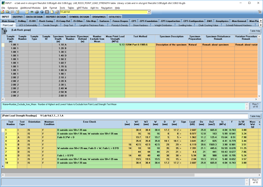
Point Load Test Table
After a record is entered for the first time and saved, the first row will automatically copy down for fields where it might be useful.
The field Number_to_Exclude_from_Is50_Mean on Point_Load_Test (upper) table defines the number of highest and lowest values to exclude from point load strength test mean (eg. If Number_to_Exclude_from_Is50_Mean is 2, the two highest and the two lowest values will be excluded for the mean calculation). The excluded tests are shown in the Exclude_From_Mean check box.The net mean is written to the Point_Load_Test (upper) table.
Moisture contents for each specimen are recorded in the Moisture_Content table.
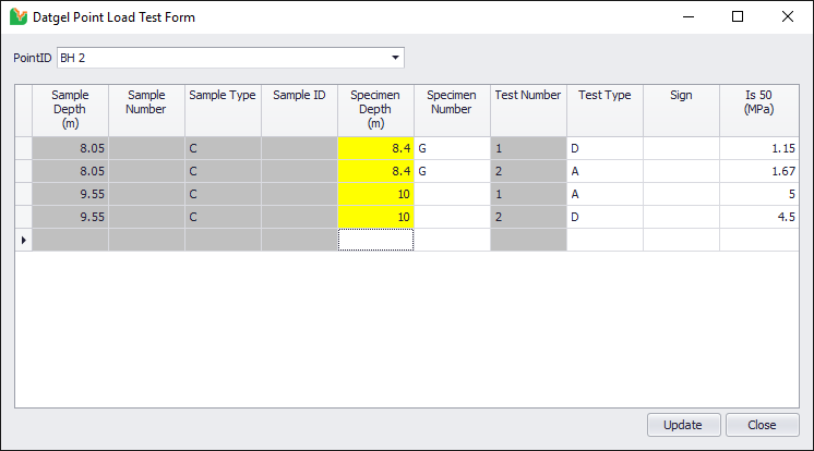
Point Load Test Form Add-In
This Tool allows you to efficiently enter Is50 results, without the need to manually create Specimen and Point_Load_Strength records.
To Launch the Tool go to INPUT and select the command Add-Ins > Datgel DGD Tool > Point Load Test Form.
The following form will then show. Select the PointID for the Point Load test results and you can view the Point Load test results for this selected PointID. You can also add a new Point Load test result for this PointID by entering the test result in the last row.
After entering a Specimen Depth, the code will define the relevant parent Sample based on the Sample Top and Bottom values and Test Number.
After you have entered the new values, click the Update button in order to save the changes into the database.
Dynamic Cone Penetrometer (DCP)
Input
IS-Comp Rel | DCP
DCP Supported Test Methods
Standard | Description |
|---|---|
AS 1289.6.3.2-1997 | Determination of the penetration resistance of a soil - 9kg dynamic cone penetrometer test |
AS 1289.6.3.3-1997 | Determination of the penetration resistance of a soil with a Perth sand penetrometer |
NZS 4402:1986 Test 6.5.2 | Determination of the penetration resistance of a soil - Hand method using a dynamic cone penetrometer |
RTA T161 | Penetration Resistance of a soil (Dynamic Cone Penetrometer - 9kg mass) |
You can have many tests in one PointID, and tests can start at any depth. The test start Depth below ground level is entered on top half of screen. The Penetration_Top/Bottom are relative to the test start Depth.
Note that although we can enter many tests in one PointID, the log reports are not designed to deal with this.
Data can be entered by Depth or Blow, as defined in Reading_Type field.
Correlations for CBR and Allowable Bearing Capacity can be calculated.
Data Entry Procedure by Depth:
- On the DCP (upper) table enter the Depth, the appropriate Type, Test_Method, Reading_Type as Depth, CBR_Analysis_Method and Allowable_Bearing_Capacity_Analysis_Method.
- When you change table, row or click save (Ctrl+S), the Hammer_Mass, Standard_Drop, Cone_Base_Diameter, Rod_Diameter, Anvil_Damper, Cone_Depth, Cone_Angle_Rod_Mass and Depth_Increment fields will also be automatically written to the DCP (upper) table. You can change the Depth_Increment field if it is necessary.
When you move to the DCP (lower) table, the Penetration_Top, Penetration_Bottom and Increment_Length fields will be automatically populated to 30 m and increasing by depth increments based on the value given in the Depth_Increment field on the DCP (upper) table.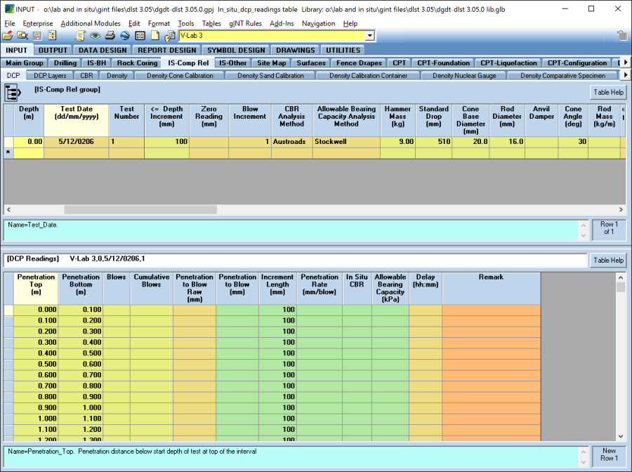
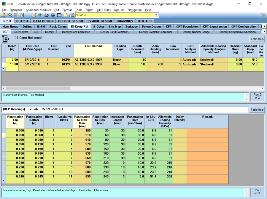
DCP by Depth Example - Enter the number of Blows for each increment. Click save (Ctrl+S) and the Penetration_Blow, Penetration_Rate, In_Situ_CBR and Allowable_Bearing_Capacity will be calculated and the Top_Depth and Increment_Length fields that have no corresponding data in the Blows field will be deleted. The Cumulative_Blows values will also be calculated.
- If the standard increment is not achieved (e.g. at the refusal depth – see Figure) then the Penetration_Bottom and Increment_Length values should be edited to show the actual increment length achieved.
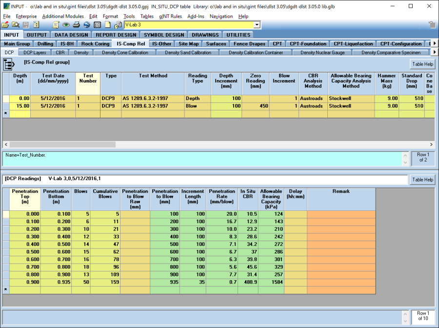
DCP by Depth Result and Refusal Example
Data Entry Procedure by Blow:
- On the DCP (upper) table set the Depth, the appropriate Type, Test_Method, Reading_Type as Blow, Zero_Reading (Initial value for Blows Calibration), Blow_Increment, CBR_Analysis_Method and Allowable_Bearing_Capacity_Analysis_Method.
- When you change table, row or click save (Ctrl+S), the Hammer_Mass, Standard_Drop, Cone_Base_Diameter, Rod_Diameter, Anvil_Damper, Cone_Depth, Cone_Angle_Rod_Mass and Depth_Increment fields will also be automatically written to the DCP (upper) table.
When you move to the DCP (lower) table, the Blows and Cumulative_Blows fields will be automatically populated. The Cumulative_Blows field will be populated to 1000 and increasing by blow increments based on the value given in the Blow_Increment field on the DCP (upper) table.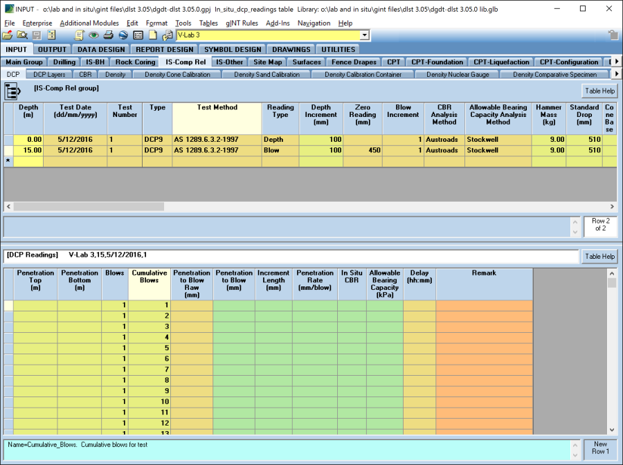
DCP by Blow Example - Enter the Penetration_to_Blow_Raw for each increment. Click save (Ctrl+S) and the Penetration_Top, Penetration_Bottom, Penetration to Blow, Increment Length, Penetration Rate, In_Situ_CBR and Allowable_Bearing_Capacity will be calculated and the Blows and Cumulative_Blows fields that have no corresponding data in the Penetration_to_Blow_Raw field will be deleted (see next figure).
DCP by Blow Result Example
The Meta data fields, such as Hammer_Mass, only calculate when the given field is empty and there are no records in the bottom half of the screen for that test.
CBR and Allowable Bearing Capacity Correlation
Correlations for CBR are included based on Austroads (2008) and RTA T161.
A correlation for allowable bearing capacity is included based on Stockwell, M. J. (1977).
Slope and y intercept for the methods are stored in library table DG_IN_SITU_DCP_ANALYSIS_METHOD, and new method can be added if it uses a straight line on a log-log plot.
Output
- Logs | IS AU BOREHOLE 3
- Logs | IS AU TEST PIT 3
- Logs | IS AU PAVEMENTS 1
- Logs | S AU PAVEMENTS 2
- Logs | IS DCP
- Logs | IS DCP 3 PER PAGE
- Logs | IS DCP WITH TEXT AND PLOT
- Logs | IS NZ SCALAR PENETROMETER
- Logs | IS NZ TEST PIT HAND AUGER 1
Lists
Lists that you expect to vary between projects are stored in the Lists table group. More fixed lists are stored in the library, as Lookup Lists, Library Data, and Symbols of various types.
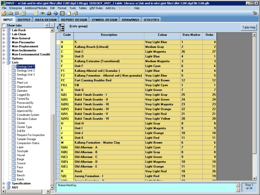
Lists group
Option Tables
The PROJECT_OPTIONS and POINT_OPTIONS tables are stored under the Options table-group.
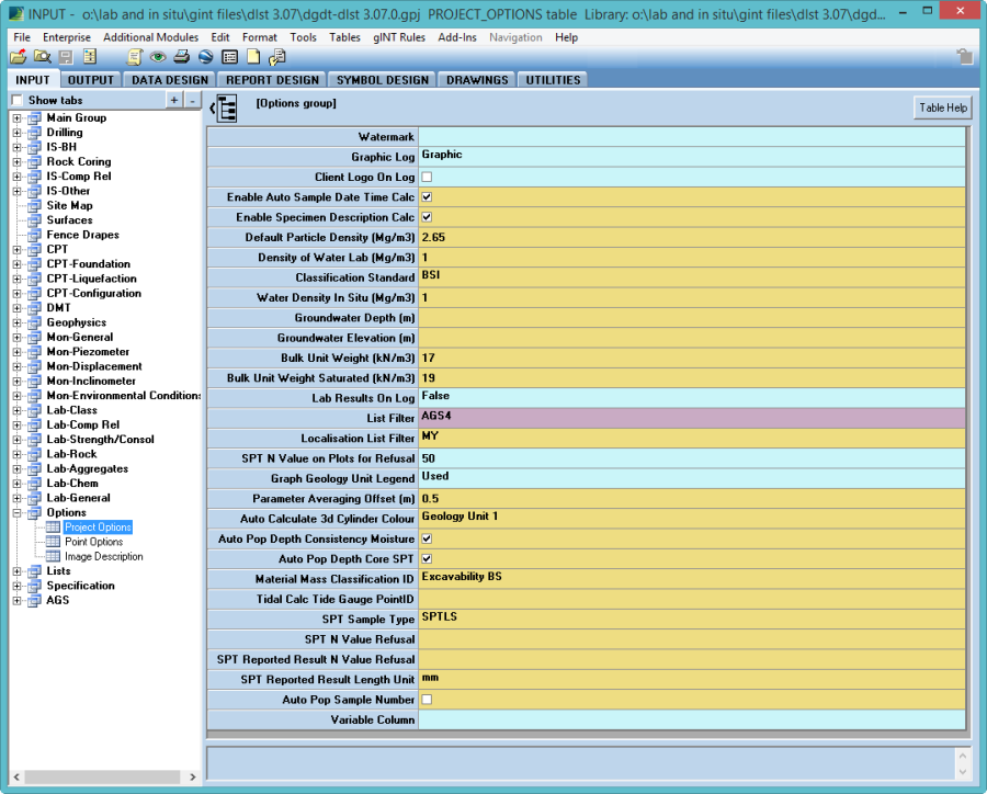
PROJECT_OPTIONS
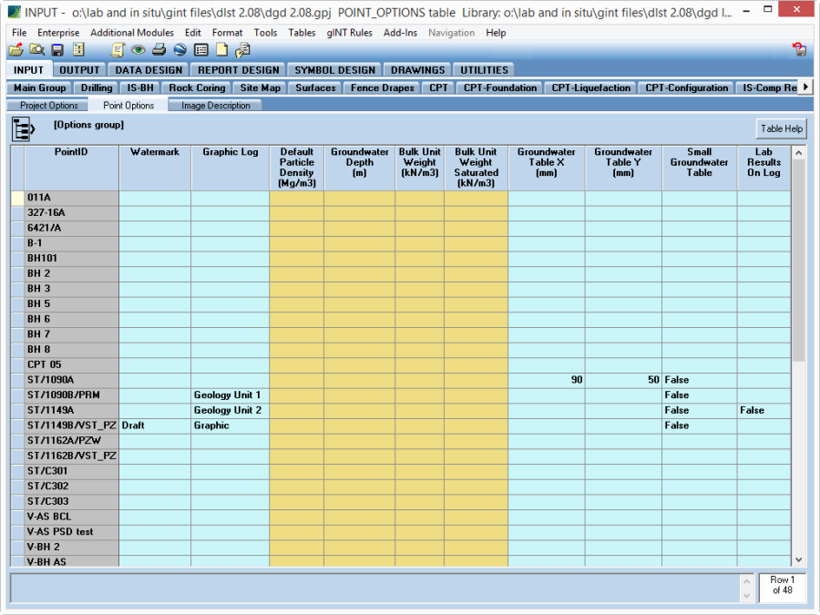
POINT_OPTIONS
If a Point level option is configured, then it will be used in precedence over the Project level option.
The Graphic_Log fields control which graphic source will be used on log reports, the options are:
- Graphic – sourced from STRATA_MAIN.Graphic
- Geology Unit 1 – sourced from STRATA_MAIN.Geology_Unit_1
- Geology Unit 2 – sourced from STRATA_MAIN.Geology_Unit_2
Site Maps
Before trying to work with Site Maps in gINT, verify that the Site Maps module has been enabled. Select Additional Modules and confirm there is a ![]() next to the Site Maps Support item.
next to the Site Maps Support item.
Importing DXF files
Drawing file type site maps are stored in the Site Maps group.
gINT only supports the import of DXF files saved in the AutoCAD Version 12 DXF file format.
To import a site map, first move to the Site Maps group, then select File > Import/Export > DXF Import, and browse to the DXF file to import.
Assuming that the information in the original DXF file was stored on separate layers, you can use the ![]() (Layer) button or the Modify > Layer menu item to display a list of the layer properties. From the window that is displayed, you can choose to Hide, Lock, change the Colour of the entities on a particular layer or Delete the entire layer; with the exception of Layer 0 which cannot be hidden or deleted.
(Layer) button or the Modify > Layer menu item to display a list of the layer properties. From the window that is displayed, you can choose to Hide, Lock, change the Colour of the entities on a particular layer or Delete the entire layer; with the exception of Layer 0 which cannot be hidden or deleted.
Import only the data and layers that you need, hence edit DXF file in a CAD software before importing. Our experience is DXF files in excess of 30 MB will cause gINT Site Map to be unusably slow.
Referencing ECW files
Geocoded Image (such as Ortho-rectified Aerial Photographs) Site Maps are also defined in the Site Maps group.
gINT only supports geocoded images that are in the Enhanced Compression Wave (ECW) file format.
Use the Site Maps group to reference a Geocoded Image. Select File > Import/Export > Import Geocoded Photo, and browse to the ECW file to reference.
You can edit the properties of the image, such as the Print Order or the Layer it is stored on, by double clicking on it to bring up the properties window. Once you have completed any required changes, click OK to save the changes (or Cancel to undo any changes) and to return to the Site Map view.
Alternatively, a less convenient way to display images in site map is using the menu item Draw > Graphics > In Place Bitmap Symbol….
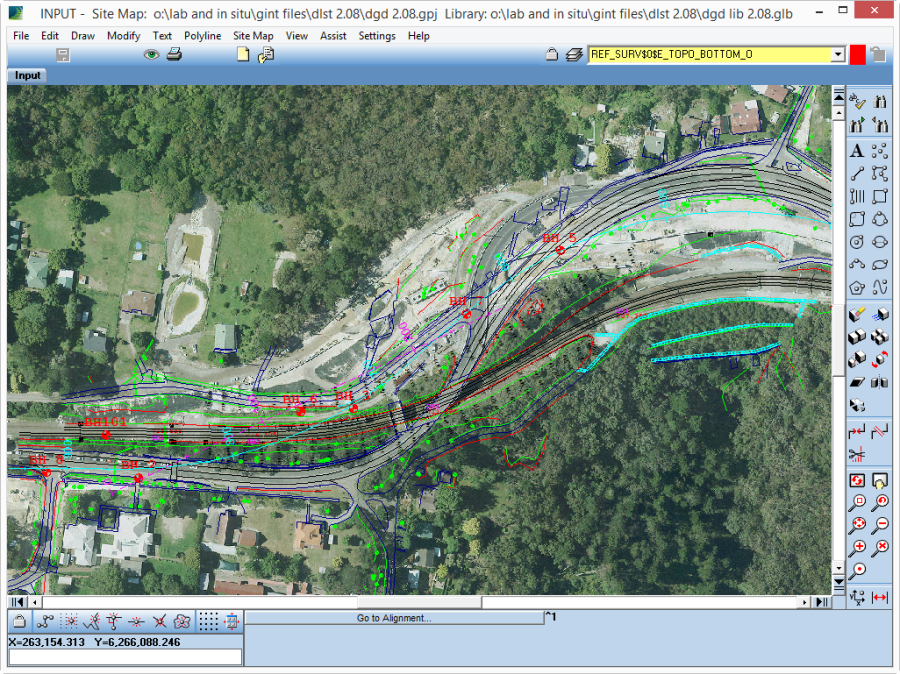
Site Map application with referenced ECW file and imported DXF
Alignments
Alignment data can be used on the Fence Reports, and to calculate chainage/offset from East/North for PointIDs.
Before trying to Import an Alignment into gINT, verify that the Alignments module has been enabled. Select Additional Modules and confirm there is a ![]() next to the Alignments Support item.
next to the Alignments Support item.
Importing an Alignment
Alignments are stored in the Main Group | Alignments table.
gINT only supports alignments that are in the LandXML, Excel or CSV file format.
To import an alignment, you should move to the Alignments table. Then select File > Import/Export > Import Alignment, and select the xml file to import.
The Alignment (upper) table contains the general information about the alignment. After an alignment has been imported, you can add additional attributes for it by selecting or entering values into the Description, Initial_Station, Alignment_Line_Type, Alignment_Line_Thickness, Alignment_Line_Colour and corresponding "Z" fields.
The "Z" lines are optionally associated with each alignment and allow for the storage of a vertical profile along the alignment. These line thicknesses are by default stored in millimetres, but you can override this by checking the Line_Thickness_in_inches field. If you do not want to display the alignment line on your site maps, check the Do_not_display_on_Site_Maps field for the relevant alignment.
The Alignment (lower) table contains the Northing and Easting values of the alignment and up to 3 optional Z values. The Station, AKA Chainage, field is read only as it is automatically populated by gINT and it records the distance along the alignment, based on the Initial_Station value in the Alignment (upper) table.
The Z fields could hold the vertical alignment, natural ground surface, or invert of a tunnel. This data also displays on the fence reports.
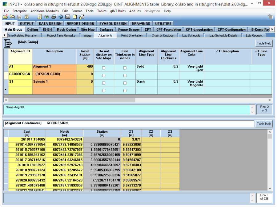
Alignments table
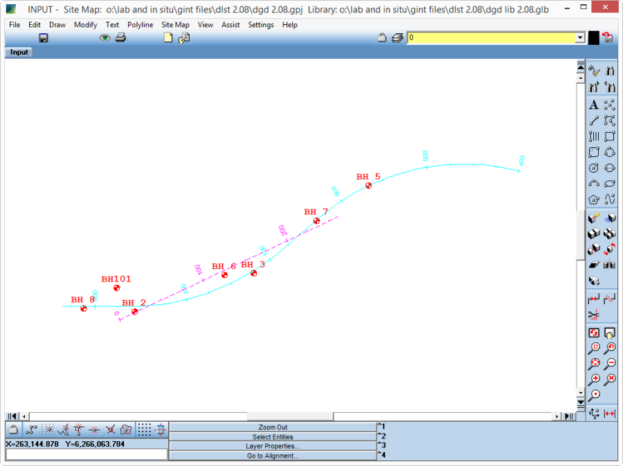
Site Map application with two Alignments
Drapes
Fence Drapes are vertical planes in 3D space, hence when viewed in plan appear as a polyline. They are commonly used to store a geophysical interpretation or a vertical profile drawing along a linear structure, and can be displayed as a projected onto a 2D Fence output. They are stored in the Input | Fence Drapes group and there is no limitation on the number of drapes that can be stored in a project file.
Before trying to import a Fence Drapes into gINT, verify that the Fence Drapes module has been enabled. Select the Additional Modules menu and confirm there is a ![]() next to the Fence Drapes Support item.
next to the Fence Drapes Support item.
Fence Drapes are a gINT Drawing object (such as an imported DXF file or image) that is stored in the project file and they are defined by a name, and the coordinates of the Drape line in plan or an associated Alignment. To add a Fence Drape to your project file, select the Input | Fence Drapes group and click the ![]() (new) icon, or select File > New.
(new) icon, or select File > New.
You should then enter a Name for the Drape and either:
- the Coordinates (as a series of East and North values) and optionally specify the Initial Station if required; or
- choose an Alignment if one already exists in your project file. This option has the advantage that the alignment is displayed in the site map, which most users will prefer.
Enter only one of Coordinates or an Alignment, not both.
The Page Size and Orientation properties are only used if printing directly from with the Drapes application.
The drapes themselves are drawn in the same way you draw any gINT Drawing object, however the scales differ:
- The X axis is the distance along the drape line
- The Y axis is defined as the elevation
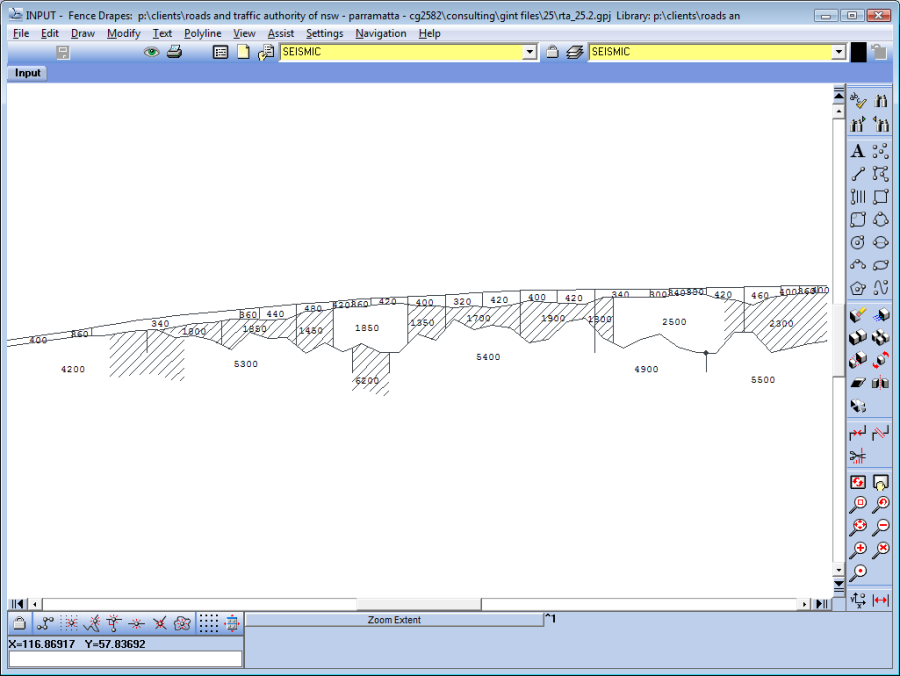
Fence Drape showing a seismic section
Importing an Image into a Fence Drape
Once you have defined the name of the Fence Drape:
- Select Draw > Graphics > In Place Bitmap Symbol.
- Click the Load Bitmap Symbol button
 to open a Windows Explorer window; where you should browse to the location of the alignment file
 - Specify either the Override Height or Override Width of the image (in metres)
- Specify the Override Horz Align and Override Vert Align of the insertion point of the image
- Define the X and Y values Align to determine the insertion point of the image relative to the Override Horz Align and Override Vert Align
To view the Fence Drape image, ensure that Show at Design Time is checked
Importing a DXF into a Fence Drape
Once you have defined the name of the Fence Drape:
- Select File > Import/Export > DXF Import. A Windows Explorer window opens, where you should browse to the location of the DXF file.
- Select the file and click Open. The drawing is imported into your gINT project file.
gINT supports DXF release 12.
Surfaces
Before trying to work with Surfaces in gINT, verify that the Surfaces module has been enabled. Select the Additional Modules menu and confirm there is a ![]() next to the Surfaces Support item.
next to the Surfaces Support item.
The Surfaces group allows you to store surface definitions, such as the ground surface level, geological unit boundaries, finial design elevation and piezometric surfaces. gINT supports both grid surfaces and TIN or DTM surfaces.
Surfaces can be displayed on Fence reports, and queried by gINT Rules.
Grid surfaces can't be generated within gINT, however data used to generate a surface representing the top of a geological unit can be exported. TIN surfaces can be generated by gINT using INPUT | Additional Modules > DTM to LandXML…, and the generated XML file can be imported into Surfaces.
Export Contour Data and Importing Grid Files
You can model a grid surface from your data by exporting it to a contouring program, such as Surfer, by using the File > Import/Export > Export Contouring Data option in the Input application.
Further information can be found on how to do this via the gINT Help file; Help > Index. Enter "Export Contouring Data" in the keyword field.
If you have already created a surface grid file, you can import it into your gINT project file.
In the simplest form the grid may be imported from a delimited XYZ file. The grid needs to be rectangular, orientated N-S/E-W, have no holes, and be perfectly regular. Grid nodes with no data must be set to 1E10 or greater.
To add a Surface grid to your project file, use the Input | Surfaces group and click the ![]() (new) icon, or select File > New.
(new) icon, or select File > New.
- Enter a Name for the surface grid and optionally add a Description.
Select the Line Type, Enter a Thickness (in inches) and select a Line Colour
The thickness of the line is in inches, and a value approximately 0.01 is appropriate.
- Click the
 Import Grid File button to open a Windows Explorer window; where you should browse to the location of the grid file
 - Click OK to import the surface file
Importing Triangulated Irregular Network (TIN) Files
gINT only supports TIN files in the LandXML file format or gINT TIN (GTN) file format.
To add a Surface grid to your project file use the Input | Surfaces group and click the ![]() (new) icon, or select File > New.
(new) icon, or select File > New.
If there is more than one TIN surface in the file that you are trying to import, gINT will prompt you to select which surface you wish to import.
- Enter a Name for the surface TIN and optionally add a Description.
Select the Line Type, Enter a Thickness (in inches) and select a Line Colour
The thickness of the line is in inches, and a value approximately 0.01 is appropriate.
- Click the Import TIN File button to open a Windows Explorer window; in which you should browse to the location of the TIN file
- Click OK to import the surface file
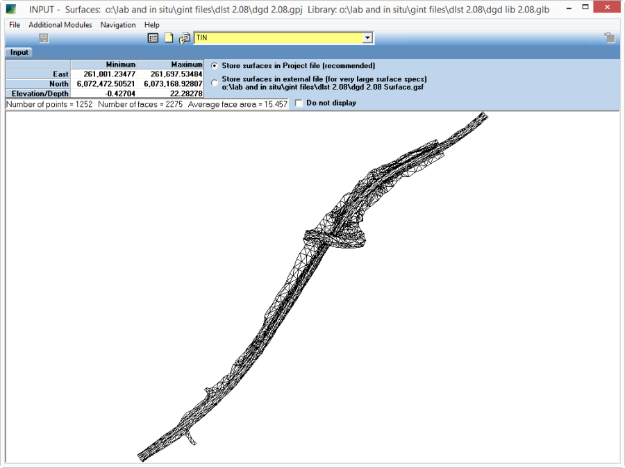
TIN Surface